What is LLM Transformer Architecture and How It Works?

By eliminating sequence-aligned recurrence, you can process entire token sequences concurrently during pretraining while maintaining direct connections across arbitrary sequence positions.

When you design high-throughput machine learning infrastructure, model scalability hinges on efficient hardware usage and long-range contextual dependencies. The structural constraints of earlier sequence transduction architectures bottlenecked parallel compute and degraded gradient signals over extended token distances.

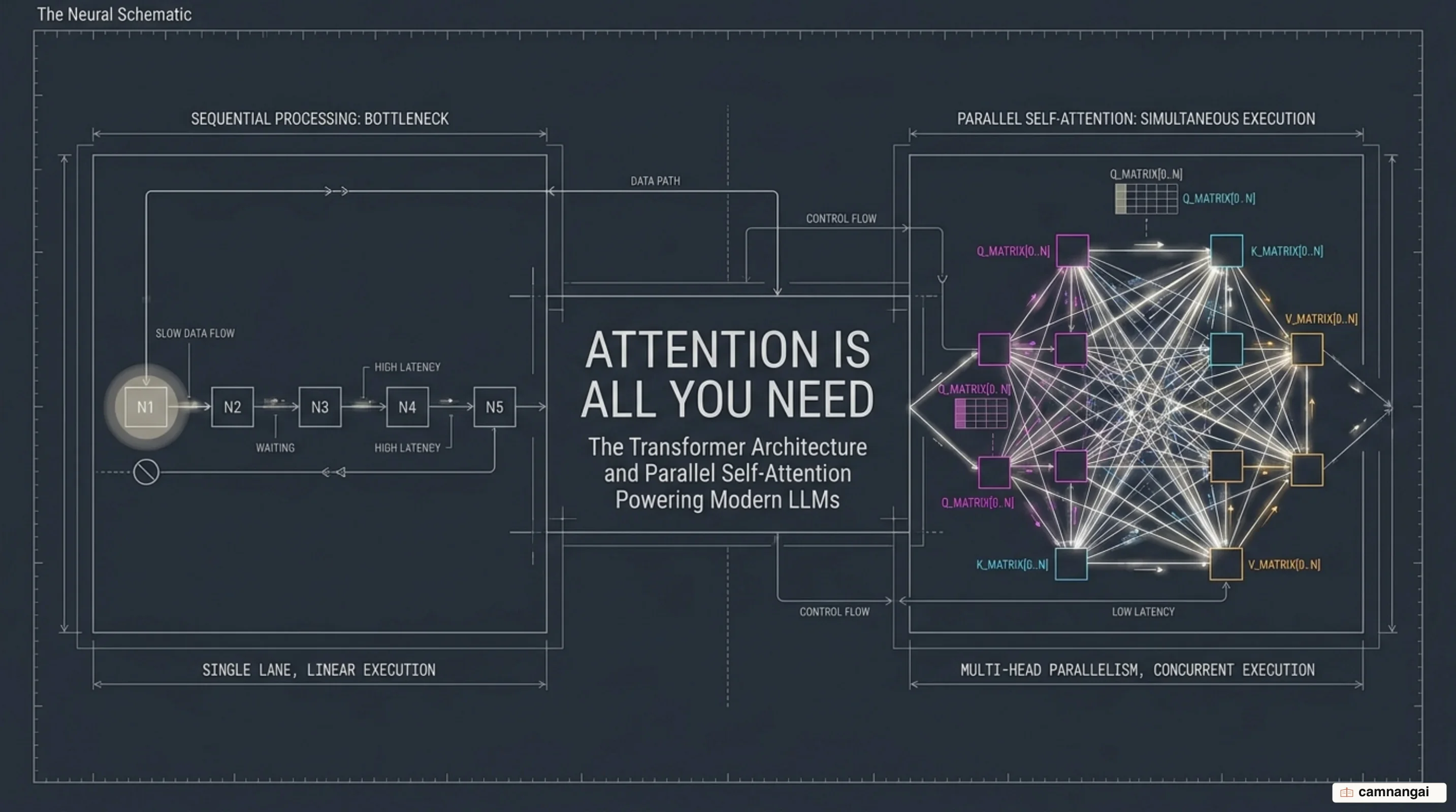
Limitations of RNNs and the Genesis of Transformers

Traditional sequence modeling architectures—such as Recurrent Neural Networks (RNNs), Long Short-Term Memory (LSTM) networks, and Gated Recurrent Units (GRUs)—factor computation along sequence positions t. To compute a hidden representation h_t, these models execute a sequential recurrence step where h_t is computed as a function of the previous hidden state h_{t-1} and the input symbol at position t. This step-by-step alignment directly ties compute time to sequence position, creating an unyielding sequential execution path.

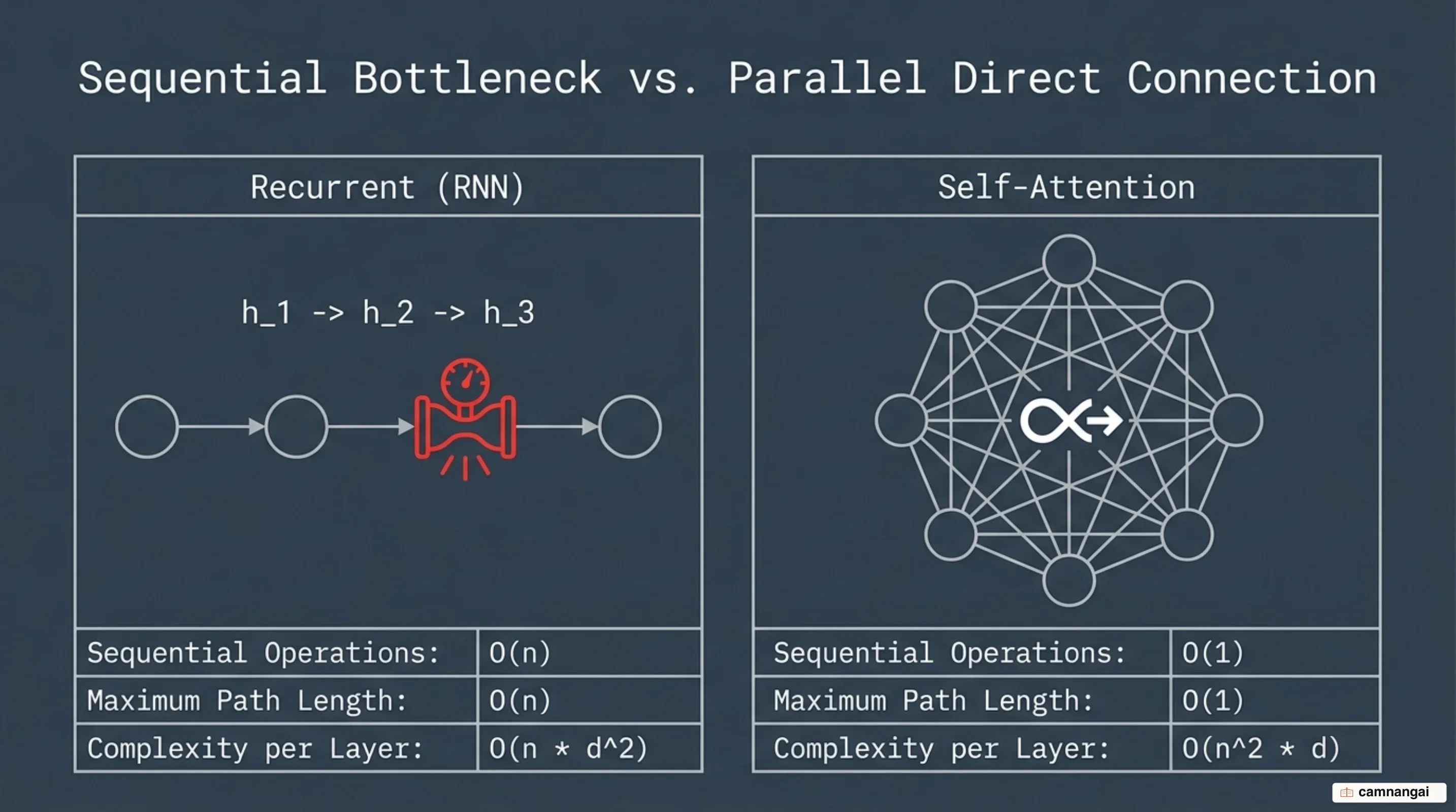
This inherently sequential design precludes parallelization within training examples. As sequence length n increases, hardware memory constraints restrict batching across examples, severely bottlenecking throughput on modern accelerator hardware like GPUs and TPUs. While computational efficiency tricks like parameter factorization and conditional compute mitigate performance overhead, they fail to resolve the underlying sequential runtime constraint.

Convolutional sequence architectures, such as ByteNet and ConvS2S, address parallelization by computing hidden representations in parallel across all input positions. However, relating signals from two distant sequence positions in convolutional models requires operations that scale linearly O(n) in ConvS2S or logarithmically O(log_k n) in ByteNet using dilated convolutions with kernel size k. This structural requirement increases the path length forward and backward signals must travel, making long-range dependencies significantly harder to learn and retain.

Self-attention in the Transformer architecture circumvents these path length bottlenecks by connecting all sequence positions in a constant O(1) number of sequential operations. At a structural level, per-layer computational complexity for a self-attention layer is O(n^2 · d), where n is sequence length and d is representation dimensionality. Compared to O(n · d^2) for recurrent layers, self-attention is computationally faster whenever sequence length n is smaller than representation dimensionality d—a condition routinely met in production subword tokenization pipelines.

High-Level Architecture: Inside the Encoder-Decoder Pipeline

The original Transformer architecture follows an encoder-decoder design. The encoder stack transforms an input sequence of symbolic representations (x_1, ..., x_n) into a continuous intermediate representation sequence z = (z_1, ..., z_n). Given z, the decoder generates an auto-regressive output sequence (y_1, ..., y_m) one token at a time, feeding previously generated output symbols back into the model as additional input for subsequent steps.

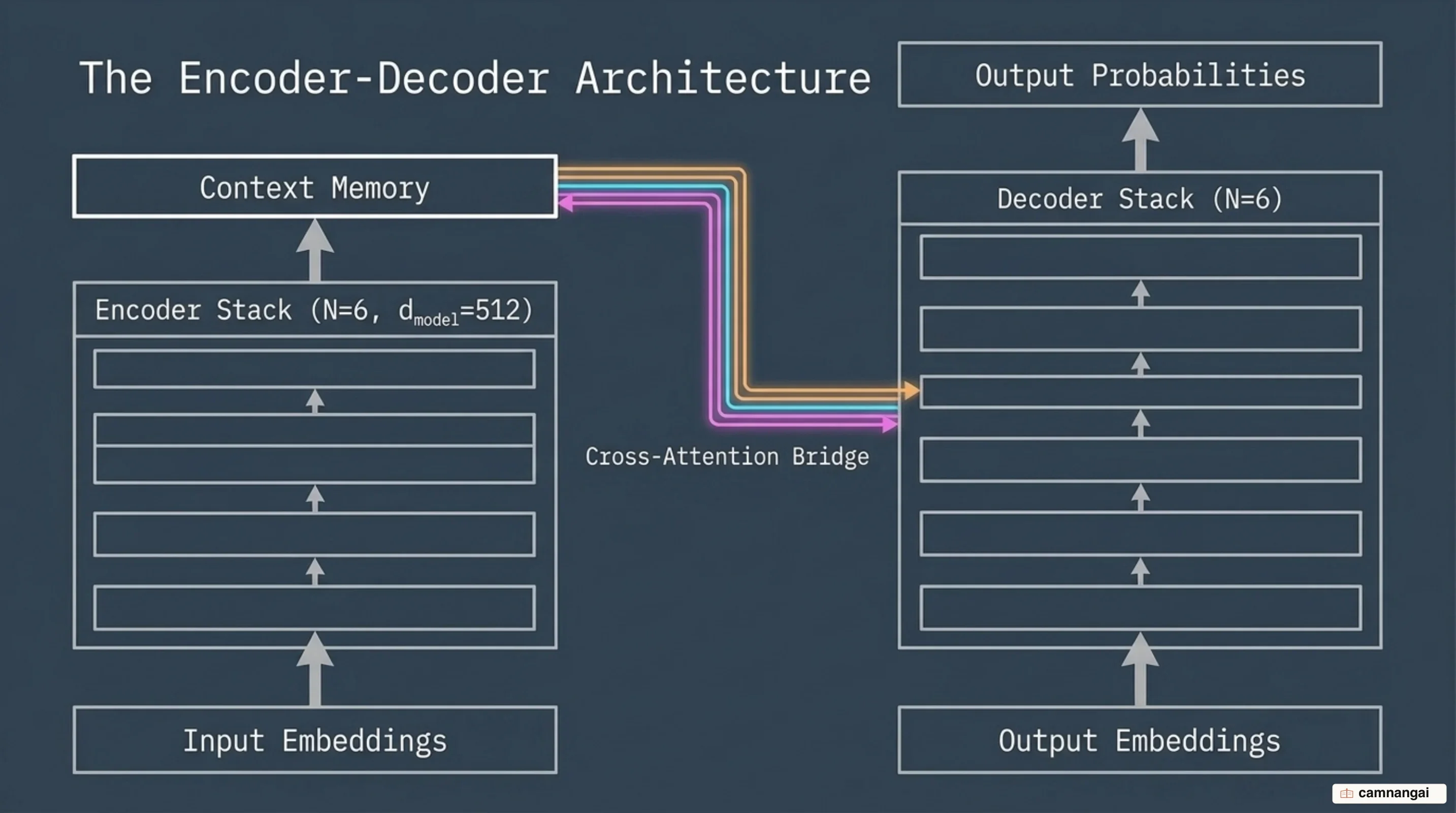
The encoder stack consists of N = 6 identical layers. Each layer contains two sub-layers: a multi-head self-attention module and a position-wise fully connected feed-forward network (FFN). Every sub-layer is wrapped with residual connections and followed by layer normalization. To ensure compatibility across residual paths, all sub-layers and embedding projections in the encoder maintain a uniform feature output dimension of d_model = 512.

The decoder stack also consists of N = 6 identical layers. In addition to the two sub-layers present in each encoder layer, the decoder inserts a third sub-layer that performs multi-head cross-attention over the output representations z of the encoder stack. Queries originate from the preceding decoder sub-layer, while memory keys and values originate directly from the encoder's output.

To maintain the auto-regressive property during training, self-attention sub-layers in the decoder incorporate target sequence masking. This masking prevents position i from attending to subsequent positions j > i by replacing unallowed attention logits with -1e9 (or -∞) before applying the softmax function. Combined with output embeddings offset by one position, this guarantees that predictions at position i depend strictly on known outputs at positions less than i.

From this core foundational design, three primary model taxonomy families emerged:

1. Encoder-only (Auto-encoding): Models like BERT that rely on bidirectional attention across all input tokens, optimizing them for sentence classification and feature extraction.
2. Decoder-only (Auto-regressive): Models like the GPT series, Llama, and Mistral that deploy causal masking across stacked self-attention blocks, optimizing them for unconstrained causal text generation.
3. Encoder-decoder (Sequence-to-sequence): Models like the original Transformer and T5 that combine distinct input encoding and auto-regressive output generation, optimizing them for conditional tasks like machine translation and text summarization.

The Mathematics of Self-Attention: Demystifying Q, K, and V

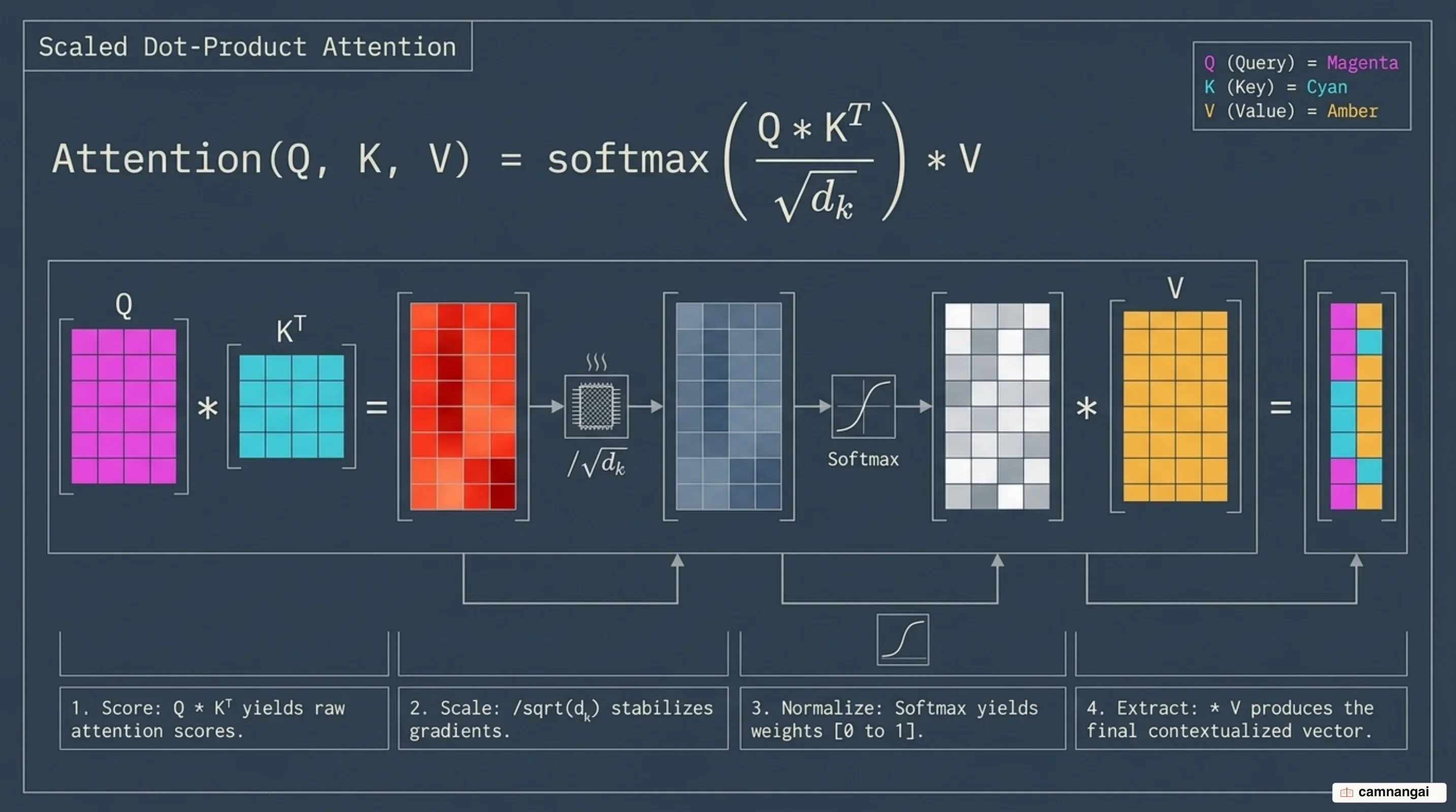
The core functional engine of the Transformer architecture is Scaled Dot-Product Attention. Input representations X are projected into three distinct tensor representations using learned linear weight matrices: Query matrix W^Q, Key matrix W^K, and Value matrix W^V:

Q = X · W^Q   (shape: [batch_size, seq_len, d_k])
K = X · W^K   (shape: [batch_size, seq_len, d_k])
V = X · W^V   (shape: [batch_size, seq_len, d_v])

The model computes attention outputs simultaneously across all packed queries via matrix operations:

Attention(Q, K, V) = softmax((Q · K^T) / √d_k) · V

The scaling factor 1 / √d_k is mathematically critical to maintaining stable gradient propagation during training. For smaller projection dimensions d_k, additive and dot-product attention perform similarly. However, as d_k grows large, the raw dot products scale proportionally in magnitude. Assuming components of Q and K are independent random variables with mean 0 and variance 1, their dot product has a mean of 0 and a variance of d_k. Without scaling, large variance pushes the softmax function into saturation regions with extremely small gradients, impeding backpropagation. Dividing logits by √d_k scales the variance back to 1.

The PyTorch snippet below demonstrates scaled dot-product attention implemented directly from scratch:

import torch
import torch.nn.functional as F
import math
 
def scaled_dot_product_attention(query, key, value, mask=None):
    # query, key shape: [batch_size, num_heads, seq_len, d_k]
    # value shape: [batch_size, num_heads, seq_len, d_v]
    d_k = query.size(-1)
 
    # Compute unnormalized attention scores
    scores = torch.matmul(query, key.transpose(-2, -1)) / math.sqrt(d_k)
 
    # Apply causal or padding mask if provided
    if mask is not None:
        scores = scores.masked_fill(mask == 0, -1e9)
 
    # Normalize via softmax to get attention weights
    attn_weights = F.softmax(scores, dim=-1)
 
    # Compute weighted context representations
    context = torch.matmul(attn_weights, value)
 
    return context, attn_weights

Multi-Head Attention: Capturing Multiple Representation Subspaces

A single attention head causes the model to average value representations over all attended positions. This averaging limits representation capacity and prevents the network from simultaneously attending to information from distinct representation subspaces across different sequence positions.

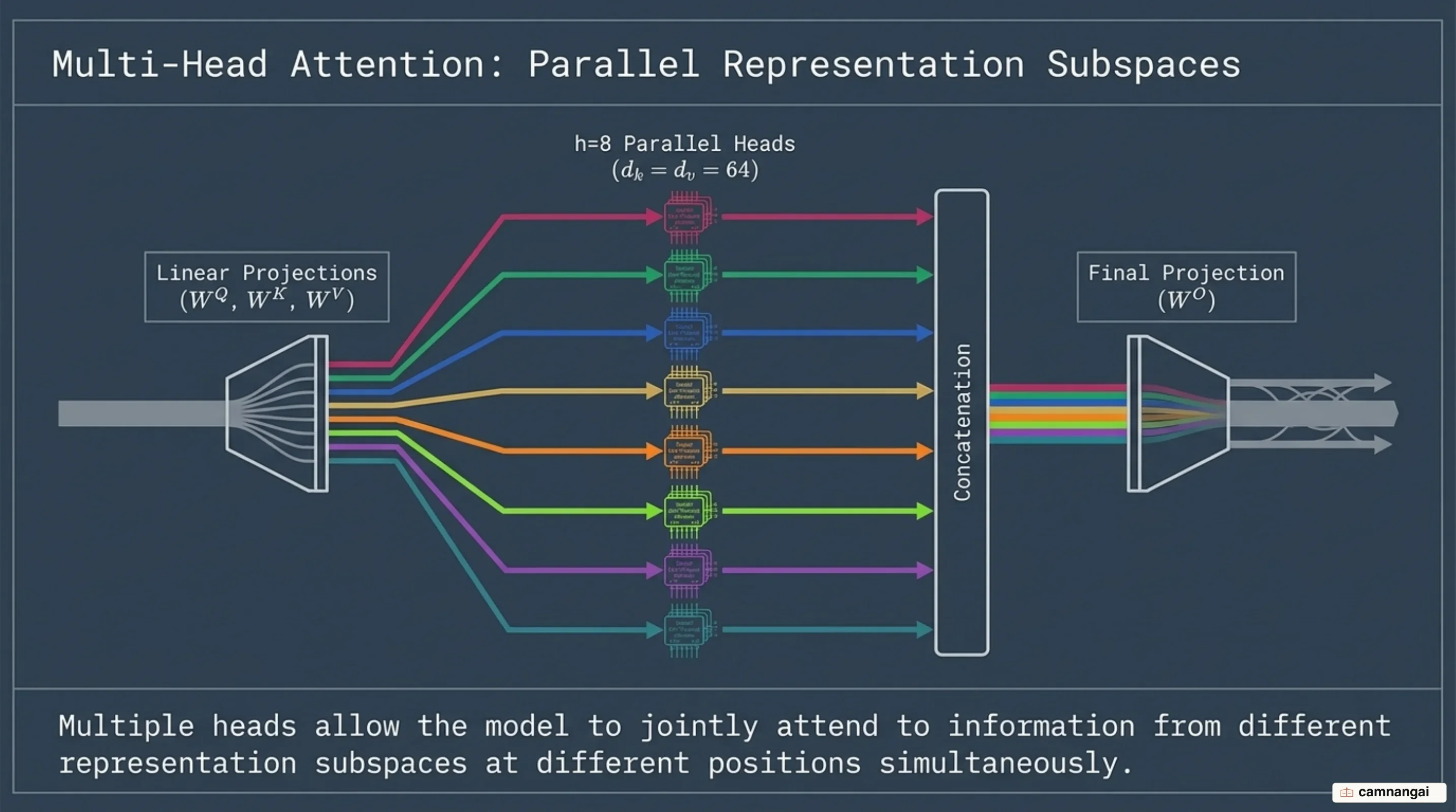
Multi-Head Attention in the Transformer architecture resolves this capacity limit by linearly projecting Query, Key, and Value representations h times using distinct, learned parameter matrices. In the baseline architecture, d_model = 512 is split across h = 8 parallel attention heads. For each head, the intermediate dimensionality is scaled down to d_k = d_v = d_model / h = 64.

The multi-head attention operation is formulated as follows:

MultiHead(Q, K, V) = Concat(head_1, ..., head_h) · W^O
where head_i = Attention(Q · W_i^Q, K · W_i^K, V · W_i^V)

The projection parameter matrices are defined as W_i^Q and W_i^K in R^{d_model x d_k}, W_i^V in R^{d_model x d_v}, and W^O in R^{h·d_v x d_model}.

To execute this operation efficiently on modern hardware, projected sequence tensors undergo explicit memory reshaping and transposition. An input tensor of shape [batch_size, seq_len, d_model] is projected to [batch_size, seq_len, h, d_k] and transposed to [batch_size, h, seq_len, d_k]. This layout allows optimized GPU tensor cores to execute batched matrix multiplication across all h attention heads simultaneously within a single GPU kernel launch, avoiding sequential loop execution overhead.

By executing scaled dot-product attention in parallel across reduced projection dimensions (d_k = 64), the total computational cost of Multi-Head Attention remains equivalent to that of single-head attention operating over full model dimensionality. This design enables individual heads to isolate distinct syntactic, semantic, and structural relationships—such as resolving anaphora or tracking distant verb-object dependencies—simultaneously.

Positional Encoding: Giving Order to Unordered Tokens

Because scaled dot-product self-attention operates as a set-based operation, the core mechanism is inherently permutation-invariant. If you shuffle input token positions without positional indicators, the resulting attention output remains identical. To give the Transformer architecture sequence-order awareness, you must explicitly inject positional signals into the input embeddings (X + PE) prior to the first layer stack.

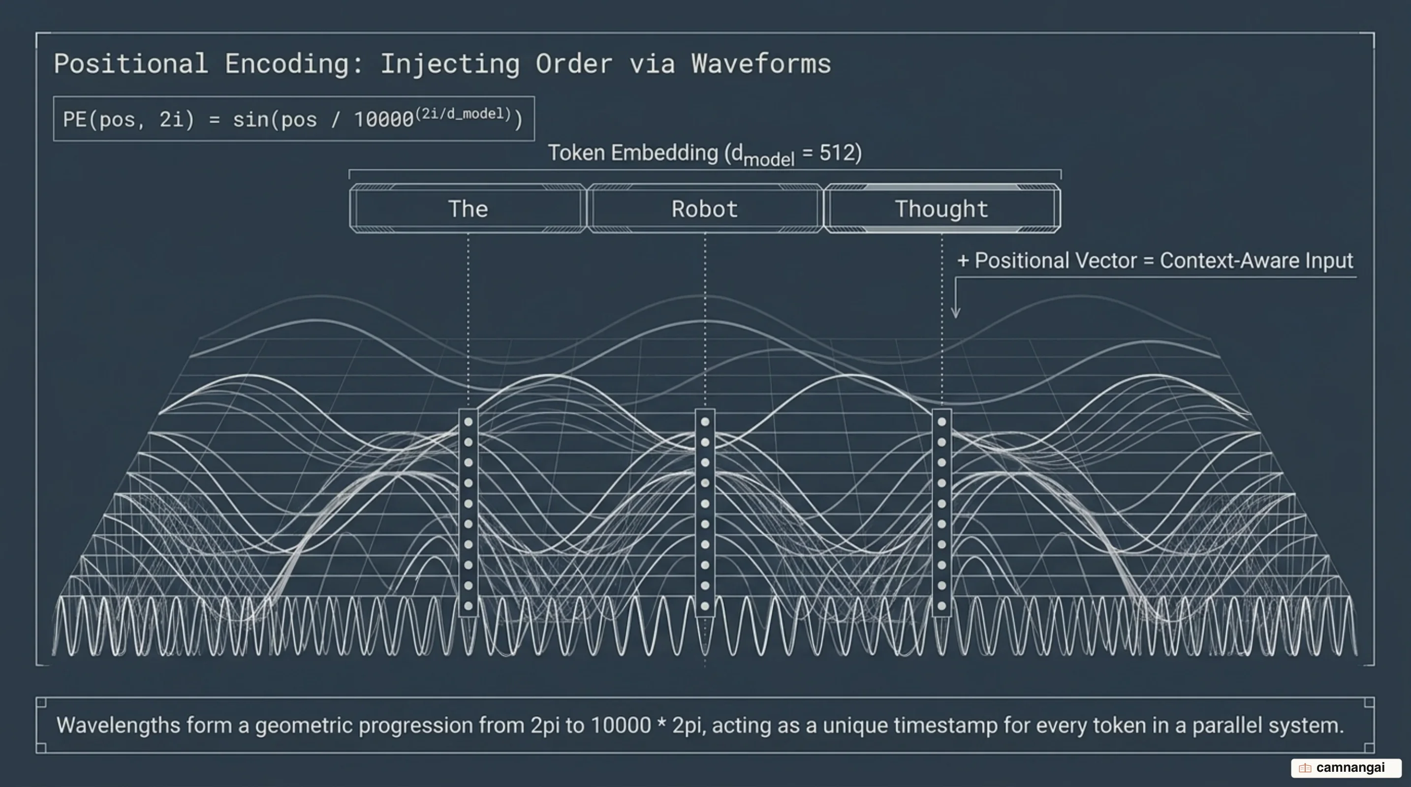
The baseline Transformer uses fixed sinusoidal positional encodings of identical dimension d_model to allow element-wise addition. The functions are defined across token position pos and dimension index i:

PE(pos, 2i)   = sin(pos / (10000^(2i / d_model)))
PE(pos, 2i+1) = cos(pos / (10000^(2i / d_model)))

The geometric progression of wavelengths across dimensions—ranging from 2π to 10000 · 2π—creates a continuous positional signal. This formulation was chosen based on the trigonometric hypothesis that the network can easily learn to attend to relative positions: for any fixed spatial offset k, PE_{pos+k} can be calculated as a linear transformation of PE_{pos}.

Learned positional embeddings represent a viable empirical alternative where positional parameters are trained alongside embedding weights. Empirical evaluations indicate that learned absolute positional embeddings and fixed sinusoidal encodings achieve nearly identical BLEU performance on baseline translation tasks. However, fixed sinusoidal encodings offer a theoretical advantage: they can extrapolate to sequence lengths longer than those observed during training.

Residual Connections, Layer Normalization, and Feed-Forward Networks

To construct stable deep networks (N ≥ 6), every sub-layer in the Transformer architecture is wrapped in a residual connection followed by Layer Normalization:

Output = LayerNorm(x + Sublayer(x))

While original architectures defined Post-Layer Normalization (LayerNorm(x + Sublayer(x))), modern LLM architectures universally adopt Pre-Layer Normalization (x + Sublayer(LayerNorm(x))). When you train deep networks with Pre-LN, gradients flow unimpeded through the main residual spine, eliminating numerical instability at deep layer counts and removing the strict necessity for delicate learning rate warmup schedules.

Layer Normalization operates across the feature dimension d_model = 512 for each token position independently, stabilizing intermediate activation distributions across training batches. In addition to attention sub-layers, each transformer layer contains a Position-wise Feed-Forward Network (FFN) applied to each token position identically and independently. The network consists of two linear transformations with a ReLU activation function in between:

FFN(x) = max(0, x · W_1 + b_1) · W_2 + b_2

where W_1 is in R^{d_model x d_ff}, W_2 is in R^{d_ff x d_model}, and the inner projection dimension d_ff = 2048 (four times d_model). This operation can also be implemented as two successive 1D convolutions with kernel size 1.

The baseline model relies on a strict regularization and optimization schedule:

• Residual Dropout: Applied to sub-layer outputs prior to residual addition and to embedding-positional sums at a rate of P_drop = 0.1.
• Label Smoothing: Implemented with ε_ls = 0.1, preventing overconfident logit outputs.
• Optimizer: Adam optimizer with β_1 = 0.9, β_2 = 0.98, and ε = 10^-9.
• Learning Rate Schedule: Warmup phase increasing linearly over the first warmup_steps = 4000, followed by inverse square-root decay.

The Shift to Decoder-Only: The Foundation of Modern LLMs

Modern large language models (LLMs) (such as GPT, Llama, and Claude) discarded the encoder stack and cross-attention sub-layers of the original Transformer, standardizing on a homogeneous decoder-only design. When you deploy decoder-only models, you consolidate the architecture into a single causal auto-regressive stack capable of processing massive text corpora with high context efficiency.

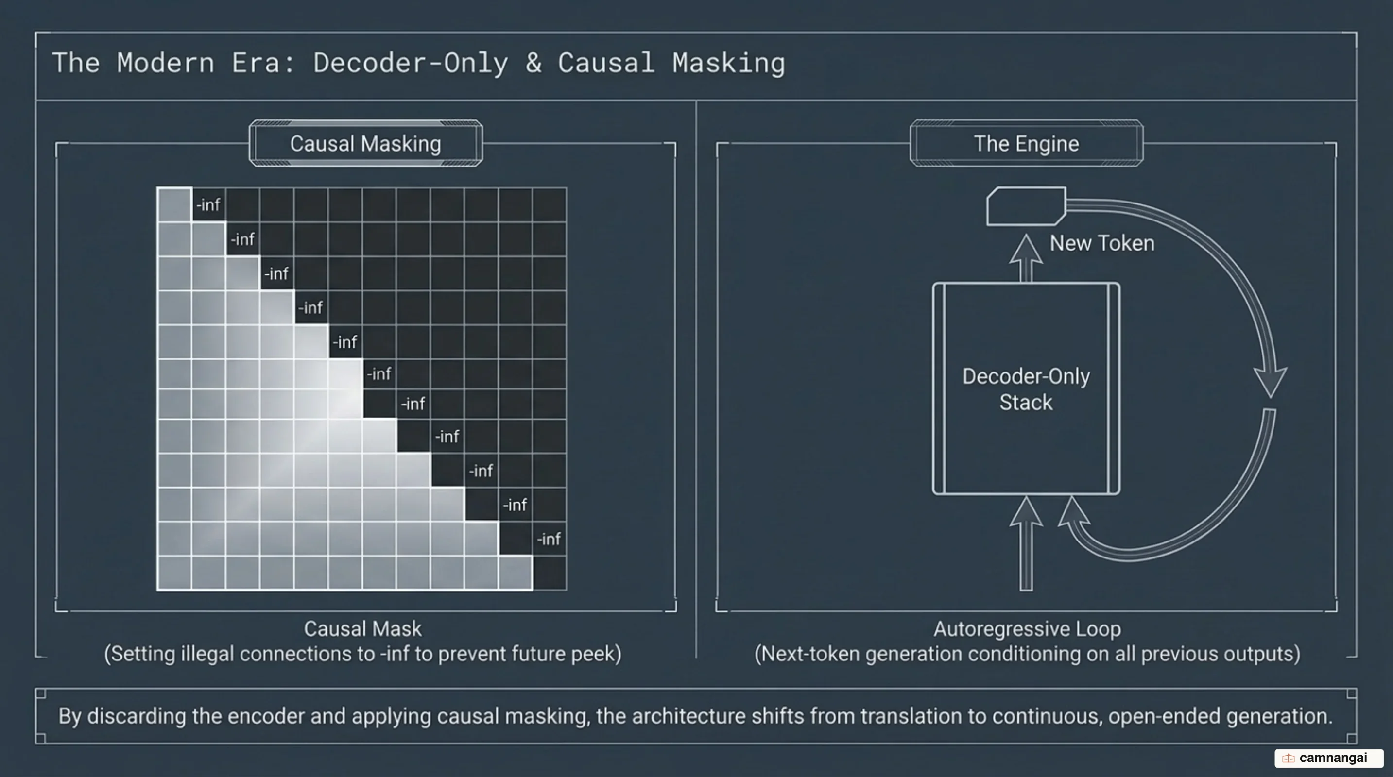
The operational workflow for auto-regressive generation in decoder-only systems follows a step-by-step execution pipeline:

1. An input token context sequence is mapped to embeddings and processed through stacked causally-masked decoder layers.
2. The final layer's output vector for the trailing sequence position is projected to the vocabulary dimension using a linear projection layer to produce raw, unnormalized logits.
3. Softmax normalizes logits into token selection probabilities, from which the next token is chosen using greedy selection, top-k, or nucleus (top-p) sampling.
4. The selected token is appended to the input context sequence, becoming the context input for the next generation step.

During pretraining, causal masking allows parallel sequence processing. By setting future attention logits to -1e9 using an upper-triangular mask matrix prior to softmax, you ensure position i cannot attend to positions j > i. This preserves causal auto-regression while allowing modern hardware accelerators to compute loss over all sequence tokens concurrently in a single forward pass.

When you manage production inference pipelines, causal generation transforms memory requirements from static weights to dynamic context buffers. Each newly generated token requires attending to historical keys and values, establishing the necessity for modern attention compute and memory optimizations.

Modern LLM Architectural Enhancements: RoPE, RMSNorm, and KV Cache

Rotary Position Embedding (RoPE) replaces static additive positional encodings by applying a rotation matrix to Query and Key representations at every attention layer. RoPE multiplies q and k vectors by a block-diagonal 2D rotation matrix, ensuring that their inner product depends strictly on relative position offset i - j. When you deploy models configured with RoPE, you achieve superior context extrapolation and preserve precise relative positional relationships across ultra-long context windows.

RMSNorm (Root Mean Square Normalization) replaces standard Layer Normalization to minimize computational overhead in deep networks. RMSNorm assumes zero-mean activation distributions and scales activations based on their root mean square alone:

a_norm = (a / RMS(a)) · g,   where RMS(a) = √( (1/d) · Σ a_i^2 + ε )

By removing the mean-centering step, RMSNorm reduces memory-bus read/write overhead on modern GPU hardware, accelerating training and inference throughput without compromising activation stability.

To optimize auto-regressive inference latency, modern architectures implement KV Caching to store previously computed Key and Value matrices in GPU memory across generation steps. Without caching, generating token S+1 requires recomputing K and V matrices for all historical context tokens 1 ... S, forcing redundant O(S^2) matrix recalculations. KV caching reduces time complexity per token generation step to O(S), but introduces massive GPU VRAM memory requirements during long-context batch serving.

To relieve this GPU VRAM footprint during auto-regressive decoding, modern LLMs transition from Multi-Head Attention (MHA) to Multi-Query Attention (MQA) or Grouped-Query Attention (GQA). While standard MHA maintains distinct Key and Value projections for every Query head, MQA shares a single KV head across all Query heads. Grouped-Query Attention (GQA)—deployed in architectures like Mistral and Gemma 2—divides Query heads into groups that share KV heads. Serving production models using GQA compresses the KV cache memory footprint in VRAM while maintaining representation quality nearly identical to full MHA.

Why the Transformer Architecture Continues to Anchor Modern AI

The Transformer architecture anchors modern AI because its constant O(1) maximum path length for long-range token dependencies pairs perfectly with modern GPU/TPU matrix multiplication hardware. By replacing sequential recurrence with parallelizable self-attention projections, you can scale training compute efficiently across massive cluster infrastructure.

While positional encodings, normalization schemes, and attention variants (such as RoPE, RMSNorm, and GQA) continue to iterate, the underlying core design—parallelizable self-attention paired with feed-forward projections—remains the foundation for production LLM deployment.

References

• Attention Is All You Need — Vaswani et al.
• The Illustrated Transformer — Jay Alammar
• The Illustrated GPT-2 — Jay Alammar
• How do Transformers work? — Hugging Face
• The Transformer Family Version 2.0 — Lil'Log
• Coding Self-Attention From Scratch — Sebastian Raschka
• The Annotated Transformer — Harvard NLP