Retrieval in RAG (Retrieval-Augmented Generation) is the architectural component responsible for querying external knowledge bases to provide a Large Language Model (LLM) with grounded context not present in its weights.
In production systems, retrieval is the primary safeguard against hallucinations by forcing the model to synthesize responses from verifiable documents rather than probabilistic next-token predictions.
The necessity of advanced retrieval stems from the limitations of static training. By integrating domain-specific, dynamic data (such as real-time technical manuals or proprietary filings), architects can bridge the gap between a general-purpose model and a specialized enterprise assistant. This process ensures that the model remains relevant without the prohibitive latency and compute costs associated with continuous fine-tuning.
As document corpora scale toward billions of entries, naive top-k vector similarity typically degrades. Information loss during embedding and the "lost in the middle" phenomenon necessitate a move toward multi-stage architectures.
For systems engineers, the challenge is no longer just finding "similar" text, but optimizing the entire pipeline for maximum precision and recall while maintaining sub-100ms latencies.
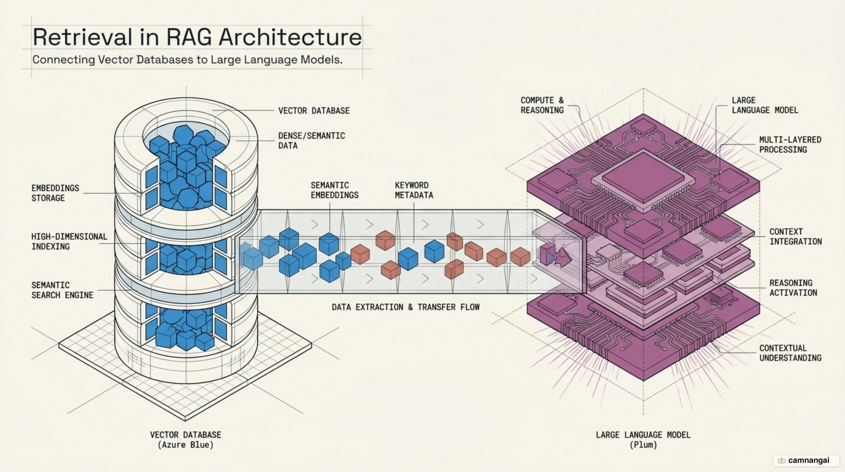
How does the retrieval process work in a RAG pipeline?
The standard retrieval flow transforms unstructured data into a searchable high-dimensional index. Documents are first decomposed into "chunks", discrete text units of a few hundred tokens. These chunks are processed by a bi-encoder (embedding model) to generate vector representations that capture semantic intent. These vectors are stored in a vector database, where they are indexed for efficient runtime proximity searches.
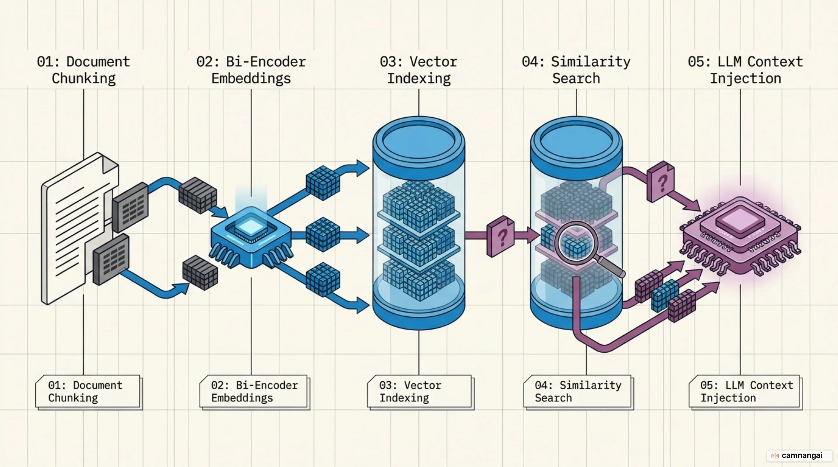
When a query is received, it is converted into a vector using the same bi-encoder. The system then executes a nearest neighbor search in the high-dimensional space to find chunks with the highest cosine similarity to the query. These results are then injected into the LLM's context window as the grounding truth for generation.
Architects must account for the "bi-encoder bottleneck." Because these models must compress the entire semantic nuance of a document into a single fixed-length vector (e.g., 768 or 1536 dimensions), significant information loss occurs. This compression makes it difficult for the system to distinguish between documents that share broad topics but differ in critical technical specifics.
Dense, sparse, and hybrid search: Why vector similarity alone falls short
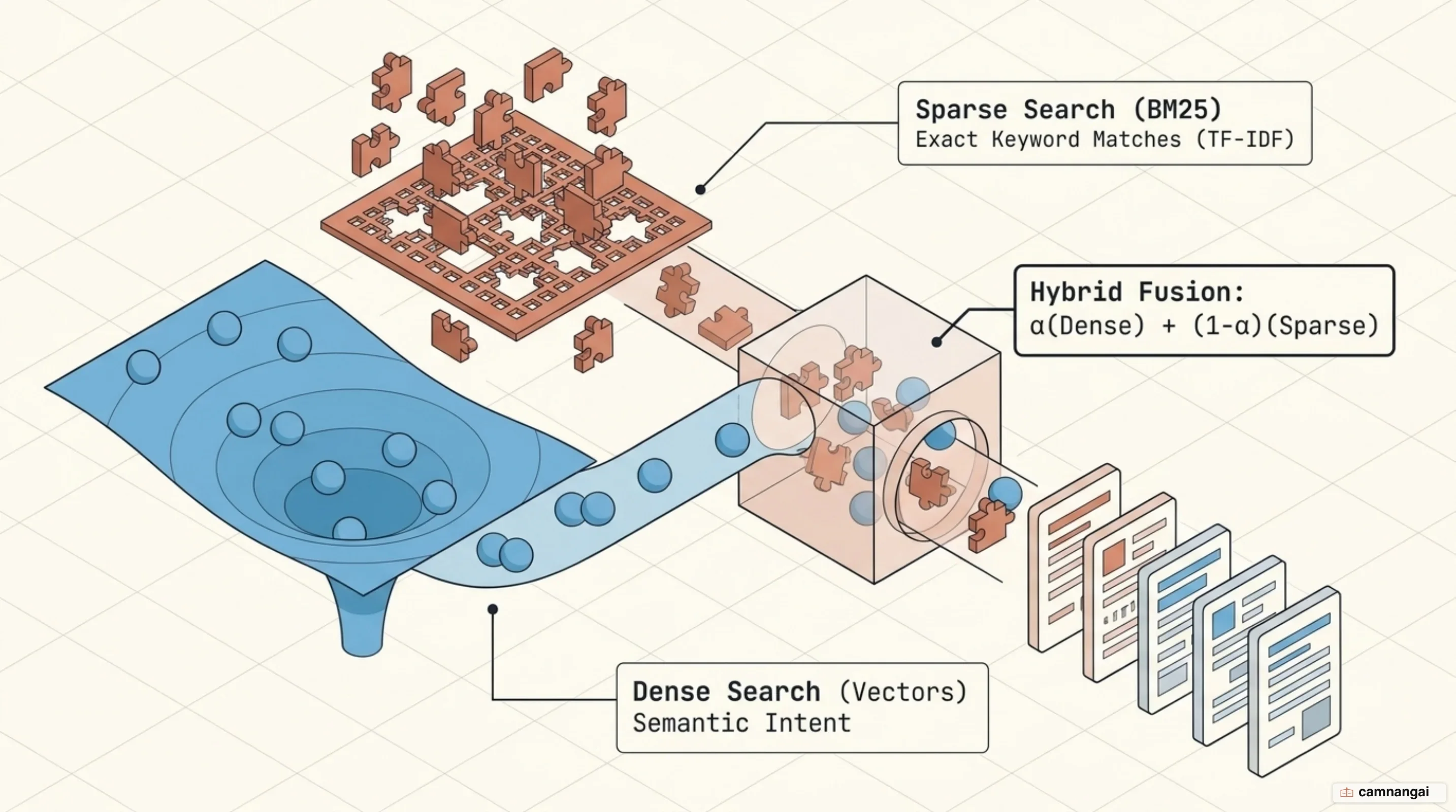
Dense vector search excels at conceptual matching but frequently fails on precise technical queries. For instance, a dense embedding might retrieve general documentation about error codes when queried for "Error code TS-999," or return general fish recipes when a user specifically requires data on "Alaskan Pollock." Sparse search (BM25) mitigates this by using lexical matching, weighing term frequency and document length to identify exact keyword matches.
Hybrid search executes both methods in parallel, merging the results via a fusion algorithm. While many systems use Reciprocal Rank Fusion (RRF), which uses the sum of reciprocal ranks to penalize lower-ranked documents, production architectures often prefer relativeScoreFusion. Unlike RRF, which discards raw scores in favor of rank, relative score fusion uses min-max normalization. This preserves the relative distance between scores, ensuring that a document that significantly outperforms others is weighted proportionally higher.
| Document | BM25 Rank | Dense Rank | RRF Score (k=0) |
|---|---|---|---|
| Document A | 1 | 3 | 1/1 + 1/3 = 1.33 |
| Document B | 2 | 1 | 1/2 + 1/1 = 1.50 |
| Document C | 3 | 2 | 1/3 + 1/2 = 0.83 |
Implementation Example
Tune the alpha parameter to balance search types. Set alpha higher (e.g., 0.8–1.0) for fine-tuned, in-domain models, and lower (0.3–0.6) for out-of-domain models where semantic mapping may be less reliable.
# Configure weight: 0.0 is pure BM25, 1.0 is pure Vector
response = index.query.hybrid(
    query="Error code TS-999",
    alpha=0.4, # Lower alpha for technical out-of-domain jargon
    fusion_type="relativeScoreFusion"
)
Approximate Nearest Neighbor (ANN) search and HNSW graph mechanics
In production, exact nearest neighbor search is too slow for million-scale datasets. We use Approximate Nearest Neighbor (ANN) algorithms, specifically Hierarchical Navigable Small Worlds (HNSW), to achieve logarithmic search complexity. HNSW builds a multi-layered structure of proximity graphs, using a probability skip list where top layers have long-range links for rapid traversal and bottom layers have short-range links for local accuracy.
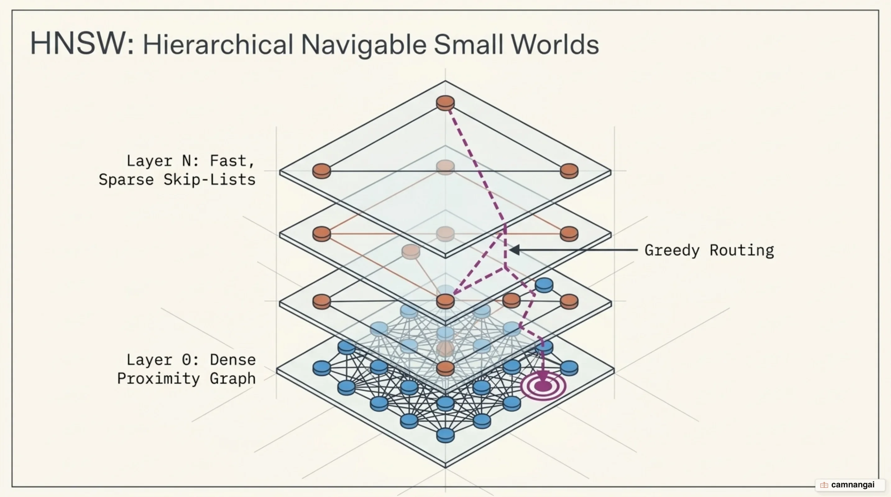
Search is conducted via greedy routing: the algorithm enters at a top-layer vertex, moves to the neighbor closest to the query, and drops to the next layer once a local minimum is reached. To maintain this structure, tune these critical parameters:
- M: Maximum number of outgoing links per vertex. Tune for memory usage; higher values increase accuracy but consume more RAM (ranging from 0.5GB to 5GB for 1M vectors). In many Faiss implementations,
M_max = MandM_max0 = M × 2(for the base layer). - efConstruction: The number of neighbors explored during index building. Increase to improve graph quality at the cost of higher build times.
- efSearch: The number of neighbors explored during a query. Increase this value to recover recall lost during the ANN approximation, though it will increase query latency.
Optimizing the pipeline: Pre-retrieval transformations and two-stage reranking
Advanced RAG requires decoupling the retrieval unit from the synthesis unit. Embedding massive chunks causes the "lost in the middle" problem, where the LLM ignores information in the center of the text.
Decoupling and Contextual Retrieval
Implement these two core decoupling strategies:
- Summary-to-Chunk: Embed high-level document summaries that link to the underlying raw chunks. This allows the system to find the right document semantically before drilling into specific details.
- Sentence-Window Retrieval: Embed individual sentences for precision, but at retrieval time, replace the single sentence with a wider window of surrounding context (e.g., +/- 5 sentences) for the LLM.
Also, use Contextual Retrieval to situate chunks. Prepend 50–100 tokens of explanatory context (e.g., "This chunk is from the Q3 tax report for ACME Corp...") to every chunk before embedding. This reduces retrieval failure rates by 35% to 49%. Using prompt caching, this situating step costs approximately $1.02 per million tokens.
Two-Stage Retrieval
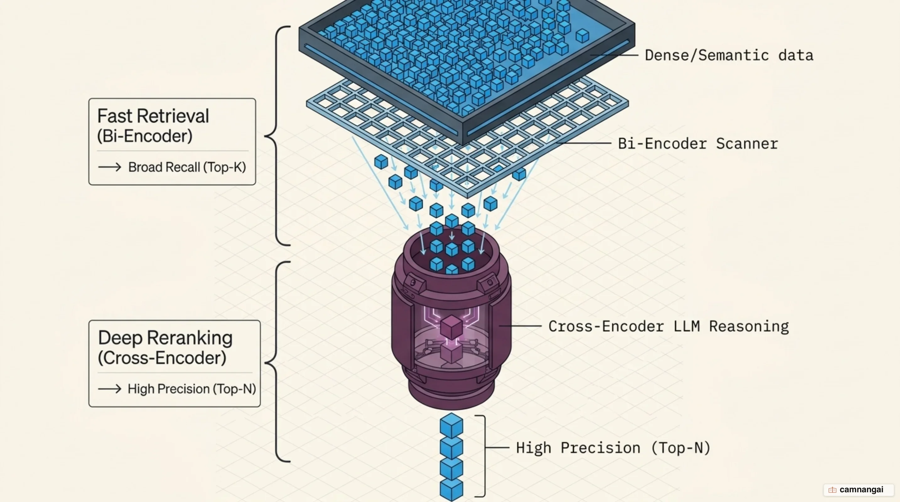
Adopt a "bi-encoder for recall, cross-encoder for precision" architecture:
- Stage 1: Use a fast bi-encoder to retrieve a broad candidate set (top 100).
- Stage 2: Pass the candidates to a cross-encoder (reranker). Unlike bi-encoders, cross-encoders analyze the query and document raw text simultaneously, avoiding the compression bottleneck.
# Initialize a local reranker for second-stage precision
from sentence_transformers import CrossEncoder

reranker = CrossEncoder("cross-encoder/ms-marco-MiniLM-L6-v2")
scores = reranker.predict([("query", "chunk_1"), ("query", "chunk_2")])
Evaluating retrieval quality: Context recall, context precision, and MRR
Evaluate retrieval success before the LLM step using quantitative metrics rather than qualitative assessments:
- Context Recall: Measures if the relevant answer is present in the retrieved set.
- Context Precision: Measures the signal-to-noise ratio and confirms if the most relevant chunks are at the top of the results, justifying the cost of the reranker.
Baseline RAG retrieval failure rates of 5.7% can be reduced to 2.9% via Contextual Retrieval, and further down to 1.9% by adding a reranking stage.
When should you upgrade your RAG retrieval architecture?
Architectural complexity should be a function of data scale. If your corpus is under 200,000 tokens, avoid the overhead of RAG and use prompt caching to fit the entire dataset into the context window. If the corpus exceeds this and includes technical jargon, transition to Hybrid Search. If accuracy remains low despite high recall, implement a two-stage reranker to filter noise and prioritize the most relevant information for the LLM.
References
- Building Performant RAG Applications for Production — LlamaIndex — Provides the primary framework for decoupling retrieval units from synthesis units via metadata replacement and recursive retrieval.
- Contextual Retrieval in AI Systems — Anthropic — Details on situating chunks and the 49% reduction in retrieval failure rates.
- Hierarchical Navigable Small Worlds (HNSW) — Pinecone — Technical deep dive into HNSW graph construction and skip list mechanics.
- Hybrid Search Explained — Weaviate — Analysis of sparse vs. dense vectors and the relativeScoreFusion min-max normalization logic.
- Introducing the hybrid index — Pinecone — Covers keyword-aware semantic search and alpha parameter weighting for in-domain vs. out-of-domain models.
- Rerankers and Two-Stage Retrieval — Pinecone — Discussion on the bi-encoder bottleneck and cross-encoder precision advantages.
- Retrieval-Augmented Generation for LLMs: A Survey — ArXiv — Academic overview of Naive, Advanced, and Modular RAG paradigms.