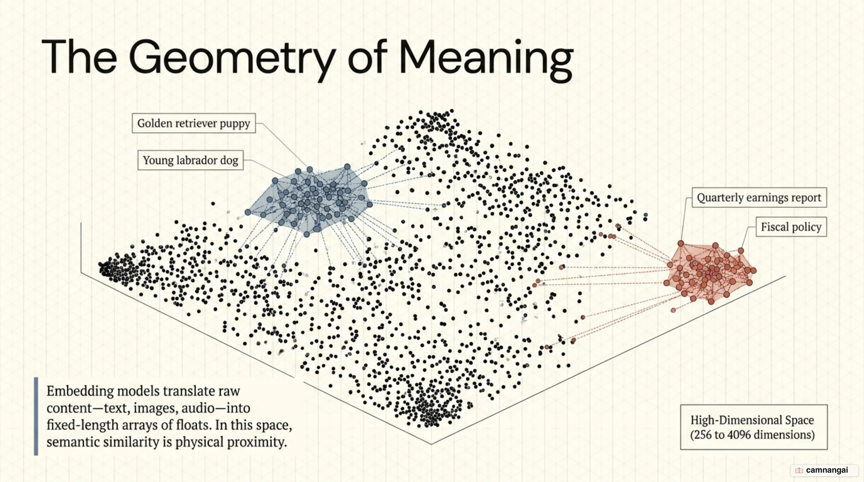
A vector database is a specialized storage and retrieval system designed to manage data as high-dimensional arrays called embeddings.
Unlike traditional relational databases that rely on exact string matches or range queries, a vector database enables similarity-based retrieval. Its primary function is to locate records that are geometrically close to a query vector in a continuous vector space rather than identifying exact textual or numeric matches.
This architectural shift is necessary for handling unstructured data such as documents, images, and audio. By mapping these inputs into a high-dimensional space, the database identifies relevant results based on their semantic proximity. This allows the system to resolve queries based on meaning — recognizing that "seafood" and "fish" are related concepts even without overlapping characters.
These databases also provide the operational guardrails you need in production. While libraries like Faiss allow for raw similarity search, a dedicated vector database provides ACID compliance, point-in-time recovery, horizontal scaling, and the ability to perform relational joins with metadata.
You are not just buying a search algorithm; you are buying the infrastructure to maintain data integrity at scale.
What is a vector database?
Traditional relational databases (SQL) are built for structured data and use B-Tree or Hash indexes to perform exact lookups. While these are efficient for integers and strings, they fundamentally fail when the query parameter is "similarity" rather than "equality." Vector databases address this by treating data objects as coordinates in a geometric space. In this approach, the distance between two points represents their semantic relationship.
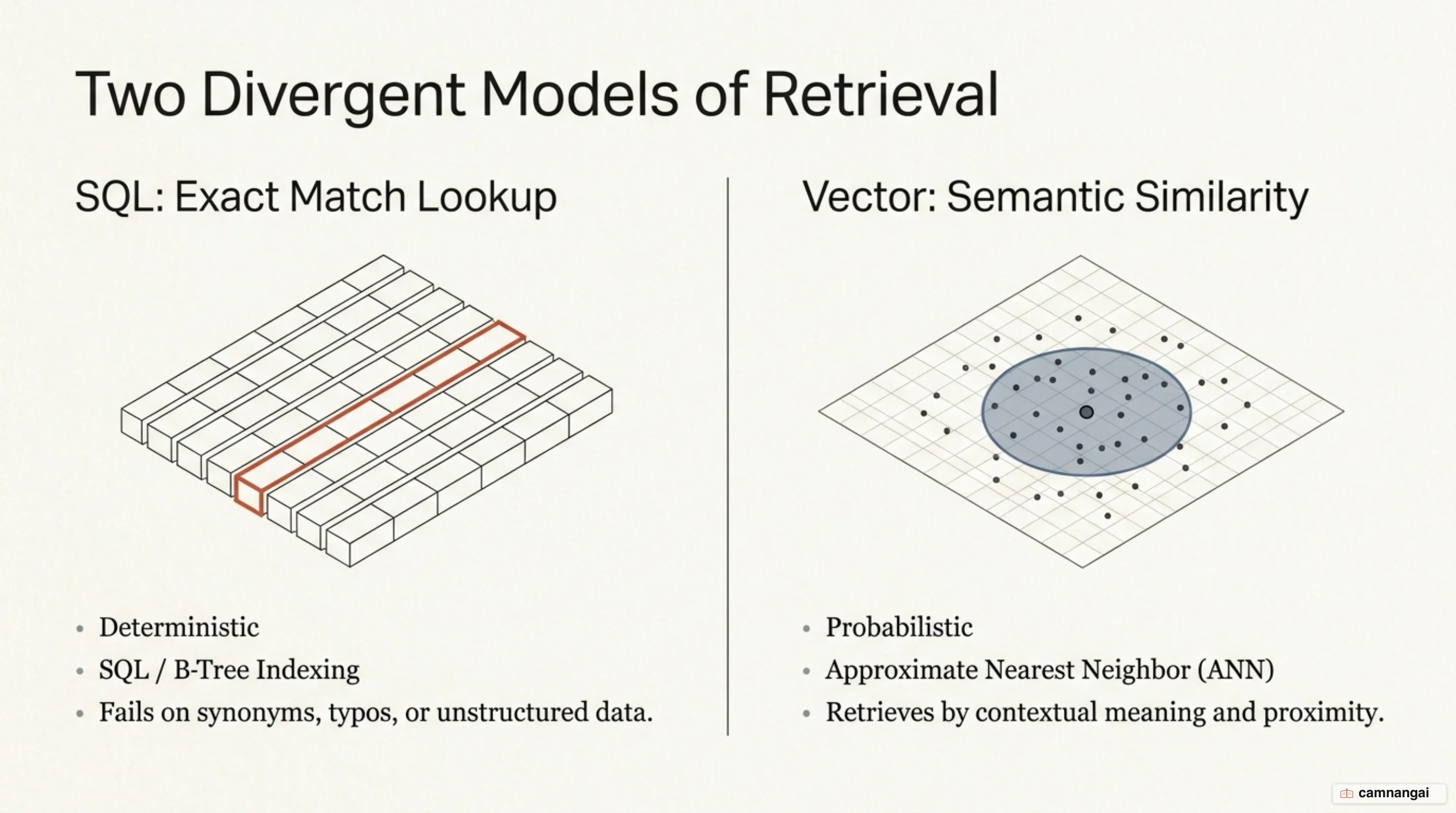
The core operation of these systems is the nearest neighbor search. In a small dataset, you could
perform a flat search (brute force), calculating the distance between a query and every stored record.
But this scales linearly — O(n) — and becomes a computational bottleneck as datasets grow. To
handle millions or billions of vectors, these databases use Approximate Nearest Neighbor (ANN)
algorithms. These algorithms provide a sub-linear search time by trading a little accuracy for a
large gain in retrieval speed.
Vector databases are a departure from traditional indexing. Where a SQL database uses B-Trees to navigate sorted lists, a vector database uses specialized geometric indexes to traverse high-dimensional arrays. This requires heavy floating-point arithmetic and specialized memory management to handle the computational load of measuring distances in hundreds or thousands of dimensions.
Beyond the search algorithm, you must consider the operational tax of the storage layer. A production-ready vector database must provide the same durability and availability features you expect from Postgres or MongoDB. This includes multi-tenancy support, snapshot-based backups, and the ability to update vectors atomically without rebuilding the entire index. These features distinguish a database from a simple similarity search library.
How data becomes a vector
Turning raw, unstructured data into a searchable format is called vectorization.
Embedding models such as OpenAI's text-embedding-3-small
or Amazon Titan Text Embeddings do this work. These neural networks encode input into a dense,
fixed-length array of single-precision floats. Depending on the model, these arrays typically range
from 256 to 4096 dimensions.
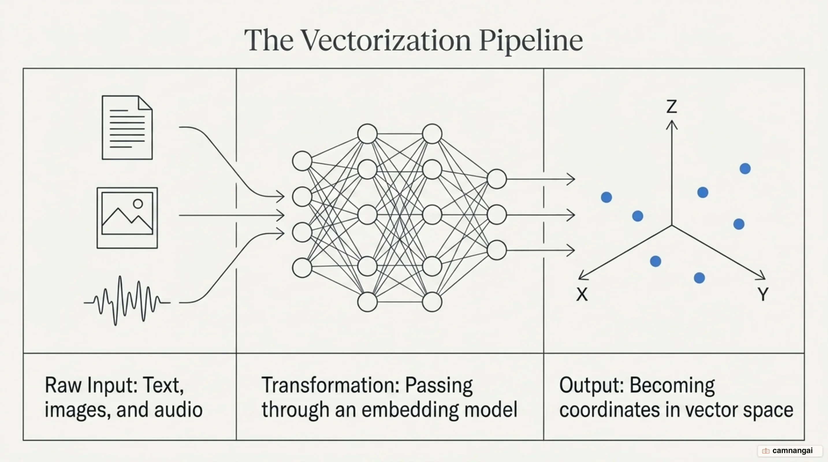
Each dimension in the array captures a specific semantic feature. While the individual floating-point
numbers are not human-interpretable, their collective position in vector space defines the data's
meaning. This geometric representation enables semantic algebra. A classic example is the operation
King - Man + Woman ≈ Queen. By subtracting the "masculinity" feature from the "King" vector and
adding "femininity," the resulting coordinates land in the neighborhood of the "Queen" vector.
When you plan infrastructure, account for the memory footprint of these floats. Vectors are stored as lists of numbers, usually 32-bit (single-precision) floats. A corpus of one million 1536-dimensional vectors requires about 6 to 7 GB of RAM for a full in-memory index. If you are operating at 10M+ vectors, you will need to consider scalar quantization or on-disk indexes to prevent memory costs from scaling out of control.
Modern embedding models are also becoming increasingly context-sensitive. Unlike early models like Word2Vec, current transformer-based models produce different vectors for the word "bank" depending on whether the surrounding text refers to a river or a financial institution. This high-fidelity representation is what allows vector databases to power complex applications like Retrieval-Augmented Generation (RAG) and recommendation engines.
How a vector database works
Distance metrics calculate similarity by measuring how close two embeddings are in high-dimensional space. The three standard metrics you will encounter are:
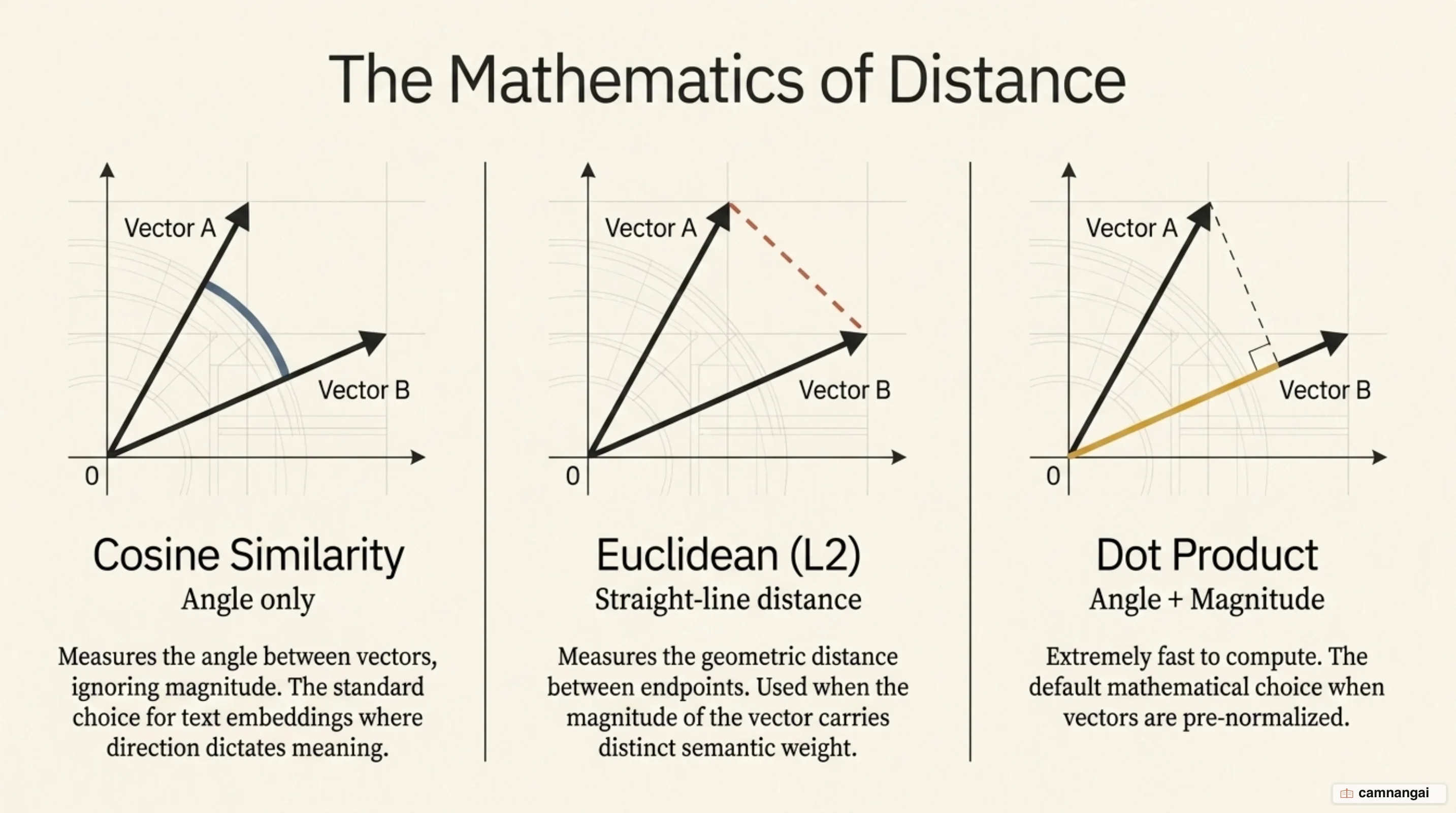
- Cosine similarity: measures the angle between vectors. It is the preferred metric for text because it focuses on the direction of the vector (the concept) rather than the magnitude (the length of the text).
- Euclidean distance (L2): measures the straight-line distance between two points. It is effective for data where the magnitude is meaningful, such as purchase counts or physical sensor data.
- Dot product: measures both direction and magnitude. This is the most computationally efficient metric, especially for vectors that have been normalized to a length of one.
Developers interact with the database via a SearchVectors API. You pass a query vector and a top-K
value, and the engine returns the K most similar results. The storage layer keeps these vectors
alongside a payload of metadata. To maintain low latency, the database holds frequently accessed
indexes in RAM, while larger datasets may use SSD-optimized storage layers like DiskANN to scale to
billions of records without requiring terabytes of memory.
In an implementation like pgvector (the Postgres extension), similarity queries use specialized
operators. For example, <=> is the cosine distance operator. A standard similarity query would look
like this:
SELECT * FROM items ORDER BY embedding <=> '[3,1,2]' LIMIT 5;When building these queries, make sure your metadata filter columns are also indexed (using
B-Trees or GIN). Without these, a filtered similarity query may degrade to a sequential scan, negating
the performance benefits of the vector index. Recent versions of pgvector (0.8+) have addressed this
by adding iterative index scans, specifically solving the recall issues where filtered results were
previously lost during the retrieval process.
Why ANN indexes like HNSW are necessary
The vector bottleneck occurs when you try to compare a query against a massive dataset. Linear scaling is a non-starter for real-time systems. To achieve sub-linear latency, most production systems use the Hierarchical Navigable Small World (HNSW) algorithm. An architectural win for HNSW is that it requires no training step — unlike IVFFlat, which requires a k-means clustering phase on a representative data sample — making HNSW far more suitable for dynamic production data.
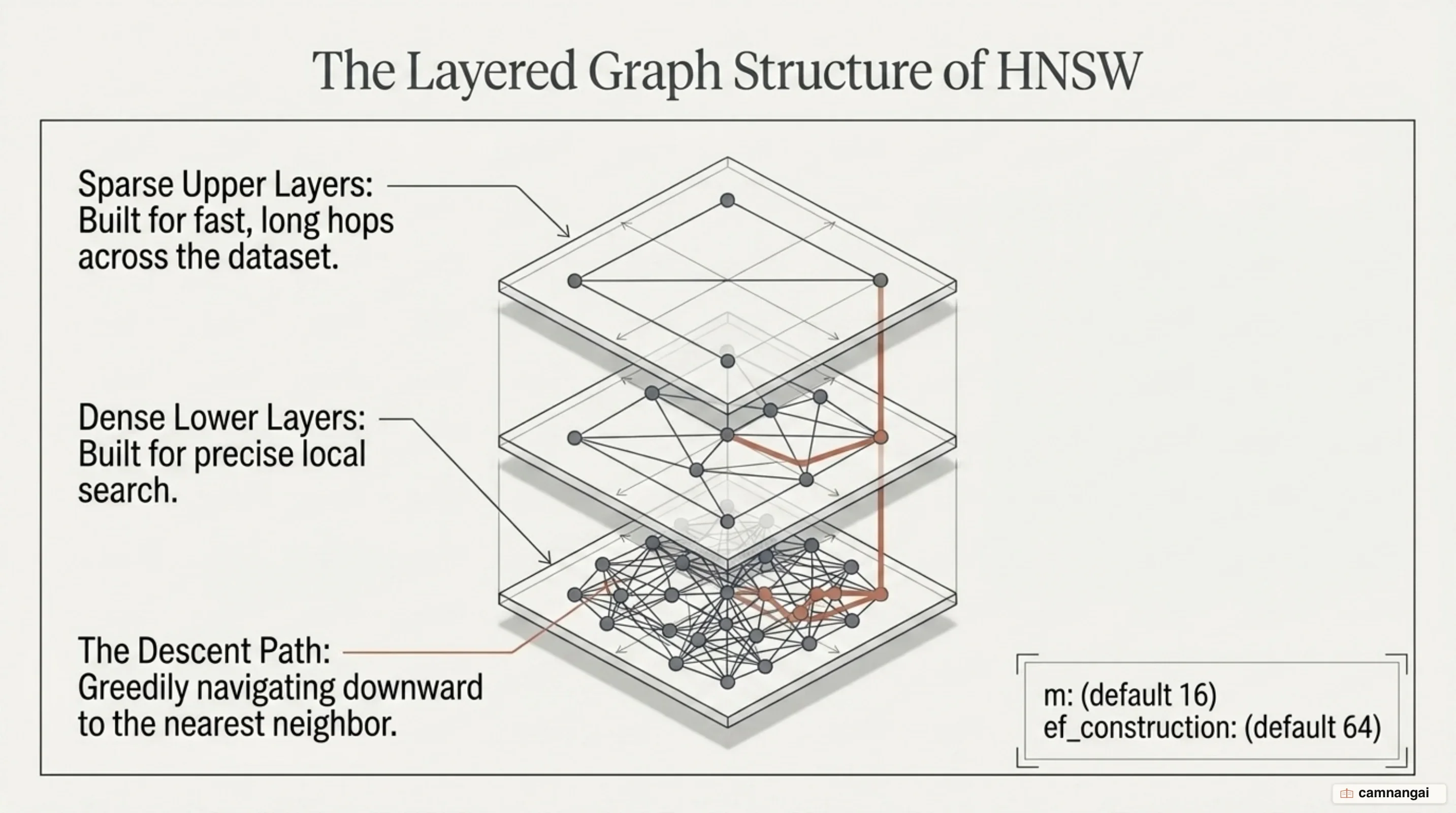
HNSW builds on the small world property, where most nodes in a graph are reachable in a few hops. The algorithm organizes vectors into a multi-layer graph hierarchy. The top layers are sparse, providing long-range, coarse hops to quickly narrow down the search region. As the search descends, layers become denser, allowing for fine-grained local search until the nearest neighbors are located at the bottom layer. While fast, this is a memory-intensive trade-off; HNSW stores multiple layers of edges, which increases the RAM overhead per vector.
Engineering teams tune HNSW using three primary dials:
- m (default 16): the number of bidirectional edges per node. Higher values increase recall and index robustness but consume more memory.
- ef_construction (default 64): the size of the candidate list during the build phase. Higher values result in a better graph at the cost of significantly longer index build times.
- ef_search: your primary recall-versus-latency dial at query time. Increasing
ef_searchimproves accuracy by exploring more candidates but adds milliseconds to your latency.
By default, HNSW provides O(log n) search complexity. But you must monitor your shared_buffers
management. In systems like pgvector, if the index exceeds the dedicated buffer pool, you will see
cache-miss latency spikes under concurrent load. Dedicated engines like Qdrant work around this by
using memory-mapped files and purpose-built I/O paths for the graph traversal.
Metadata filtering and hybrid search
A common production failure is the pre-filtering versus post-filtering problem. Post-filtering runs the
ANN search first and applies filters (for example, price < $100) to the results. This often leads to
missing results — if your top 100 vector matches are all over $100, the user gets zero results even if
valid items exist further down the list. Pre-filtering applies constraints first but often breaks the
ANN index's efficiency.
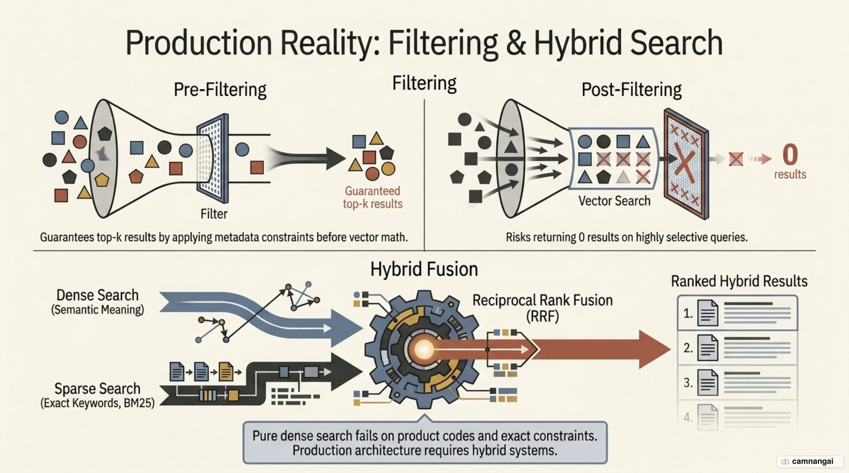
To solve this, modern engines like Qdrant use payload-indexed HNSW. In this architecture, the HNSW
graph is metadata-aware; the traversal itself respects the constraints, ensuring you get the requested
top-K results without the performance penalty of a sequential scan. This is critical for multi-tenant
applications where every search must be scoped to a specific tenant_id to maintain isolation and
performance.
To increase precision, teams are moving toward hybrid search. This combines dense search (semantic similarity) with sparse search (keyword matching like BM25). Dense vectors excel at general meaning but fail at exact constraints like part numbers or specific proper nouns. These two result sets are fused using Reciprocal Rank Fusion (RRF). RRF is the industry standard because it is parameter-free and robust, allowing you to combine semantic and keyword scores without the manual alpha tuning required by weighted linear combinations.
Amazon DynamoDB's vector search adds another useful pattern. You can use partition keys to scope a search. By pinning a vector search to a specific partition — such as a marketplace or a specific user ID — you can maintain single-digit millisecond latency even as the global index grows to trillions of vectors. This scoping prevents the global search overhead for queries that are naturally constrained by business logic.
Where vector search falls short
Vector search has a fundamental limitation rooted in sign rank theory. Single-vector models struggle
with geometric partitioning — the mathematical inability of a d-dimensional vector to effectively
partition a space of n documents for complex, compositional queries. The theoretical constraint is
rank(B) ≤ d, meaning a vector can only hold so much information before intents are averaged out.
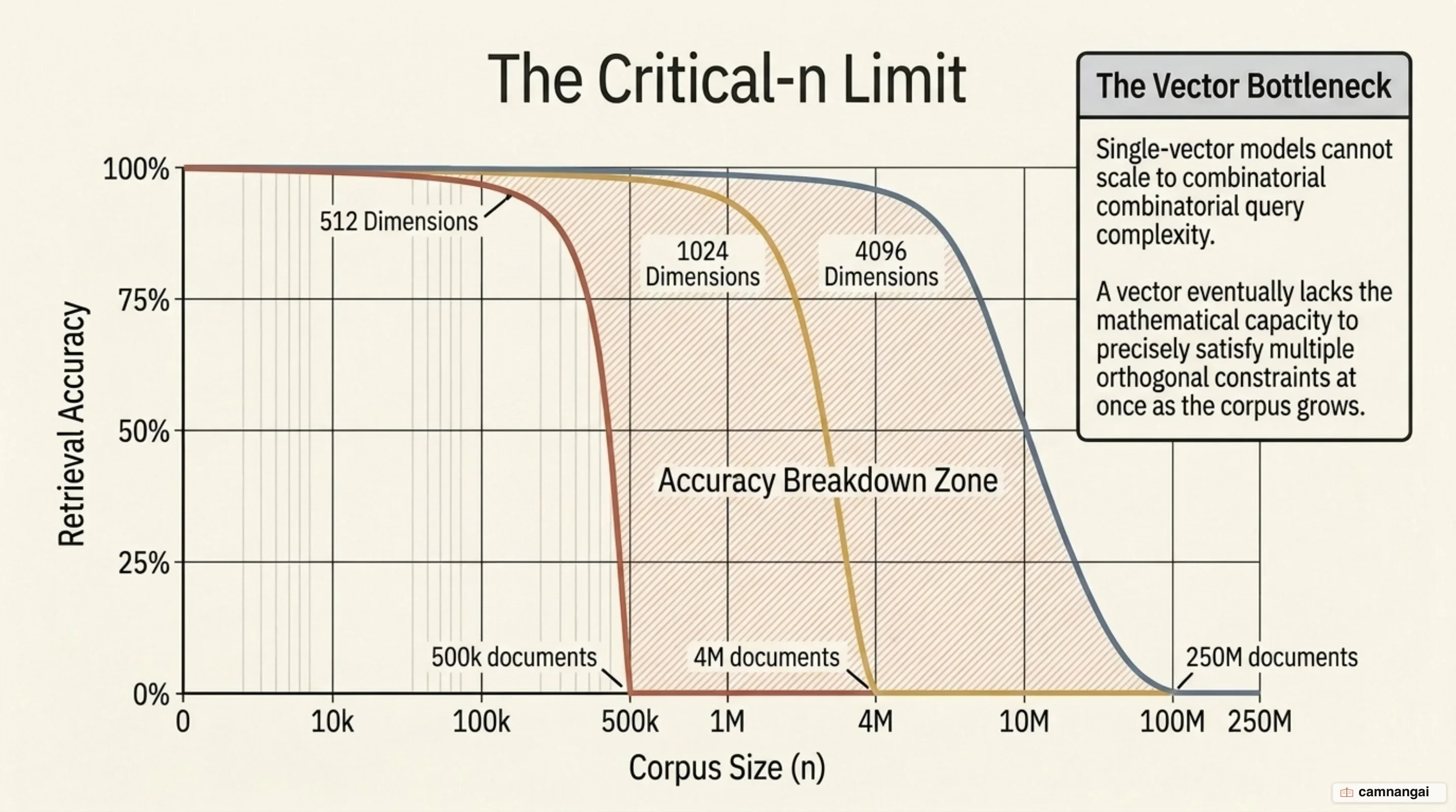
This leads to the critical-n point failure. DeepMind's work on the vector bottleneck puts a number on
it: a d=1024 model begins to fail on combinatorial tasks once the corpus exceeds about 4 million
documents — and a d=512 model breaks
down an order of magnitude earlier, at around 500,000. For example, a query like "Compare FDR and
Reagan's fiscal policies" asks for two distinct sets of evidence. A single-vector model often
retrieves a document that mentions both shallowly, rather than the best individual documents for each
president, because it tries to find a single point in space that satisfies two orthogonal intents.
Vector search is also inherently lossy. Compressing a 50-page document into a single 1536-dimensional point averages out fine-grained details. This is why complex retrieval tasks often require multi-vector models (like ColBERT) or secondary rerankers. Without these, you lose the precision needed for needle-in-a-haystack queries where a specific, non-semantic detail matters more than the overall theme of the document.
Vector search also fails at exact boolean constraints. If a user needs exactly five items under $100, the geometric proximity of vectors does not naturally satisfy that logic. You cannot rely on the vibe of a vector to enforce business rules. You must layer metadata filtering on top of the vector search to handle exact numerical or categorical requirements.
Do you actually need a dedicated vector database?
Choosing the right architecture comes down to scale and operational capacity. Treat adding a new database to your stack as a significant operational tax, and only do so when your existing tools fail to meet performance requirements.
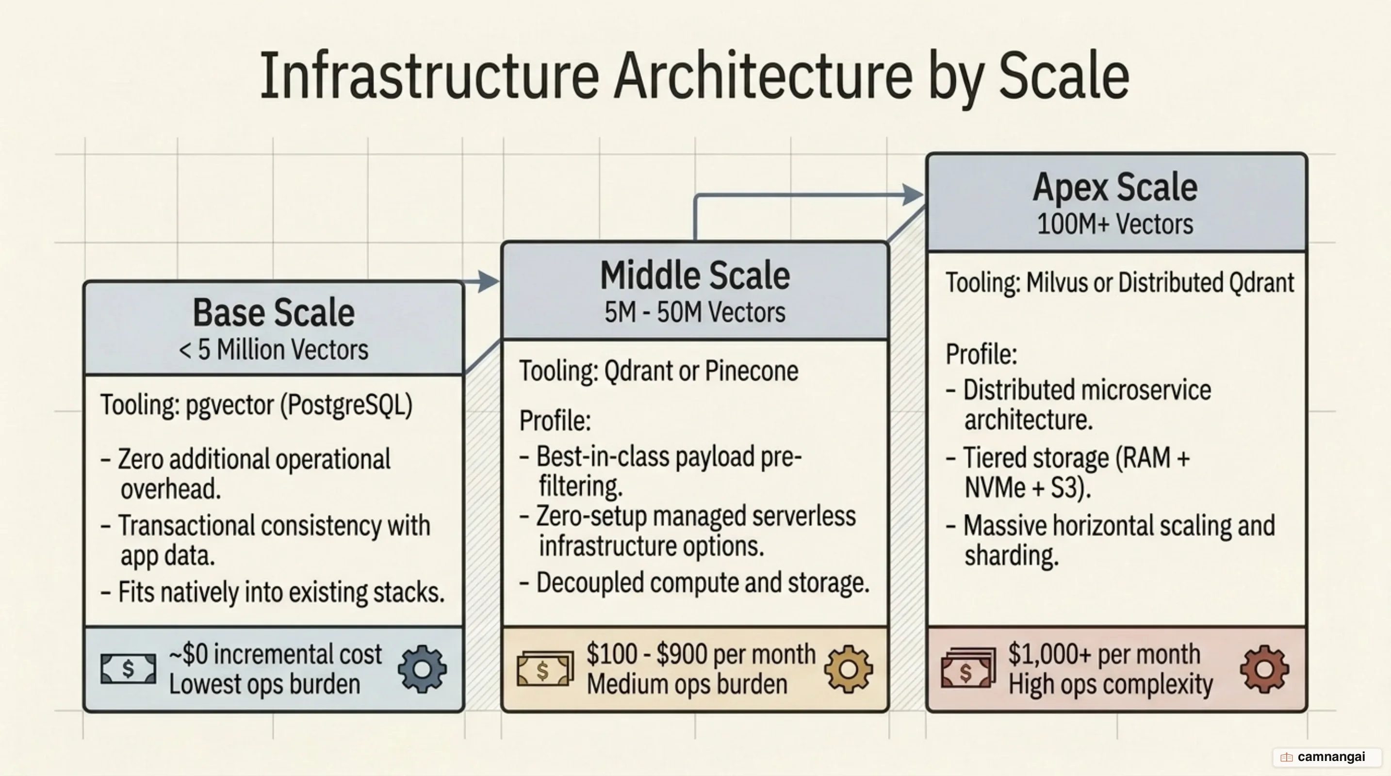
- Under 5M vectors: use
pgvectoror DynamoDB. Keeping vectors within your existing transactional boundary is almost always the correct move. It eliminates data sync pipelines and allows you to use your existing backup and security protocols. - 5M to 50M vectors: dedicated engines like Qdrant or Weaviate become economical. They offer better RAM management (like scalar quantization) and faster filtered retrieval. The crossover point usually occurs when your managed database costs hit $300–$500/month; at this stage, the performance gains of a specialized engine justify the infrastructure complexity.
- 100M+ vectors: you require distributed architectures like Milvus. These systems are designed for high write-throughput and use tiered storage (S3/NVMe) to manage datasets that cannot possibly fit in a single node's RAM.
Managed services like Pinecone are excellent for zero-ops prototyping and moving fast. However, for teams with existing Kubernetes expertise, self-hosting can cut the bill sharply: one documented migration from Pinecone to Qdrant at 8M vectors reduced monthly infrastructure cost by 72%. The decision hinges on whether you have the engineering hours to manage rolling upgrades and shard rebalancing, or if you prefer to trade a higher monthly bill for managed simplicity.
Where to start
Do not over-engineer early. If you are already running Postgres, start with the pgvector extension.
It allows you to build your first RAG pipeline or recommendation engine without the overhead of a new
data sync service. Keeping your vectors and relational data in the same transaction boundary is a big
win for early-stage development.
As your system matures, watch for semantic drift and monitor your recall metrics. Once you hit the critical-n point, or your latency requirements demand specialized filtering, then you can justify migrating to a dedicated engine. Always implement an evaluation pipeline first; if you can't measure your retrieval quality, switching databases won't solve your precision problems.
References
- What is a Vector Database & How Does it Work? Use Cases + Examples — Pinecone
- Vector Embeddings Explained — Weaviate
- Vector Databases Explained in 3 Levels of Difficulty — MachineLearningMastery
- Understanding Hierarchical Navigable Small Worlds (HNSW) for Vector Search — Milvus
- pgvector: Open-source vector similarity search for Postgres — GitHub
- pgvector Guide: Vector Search and RAG in PostgreSQL — Encore
- The Vector Bottleneck in Embedding-Based Retrieval — Tullie Murrell
- Vector Database Comparison: Pinecone vs Qdrant vs Weaviate vs pgvector in Production — Tensoria
- Amazon DynamoDB now supports real-time vector search at any scale — AWS News Blog