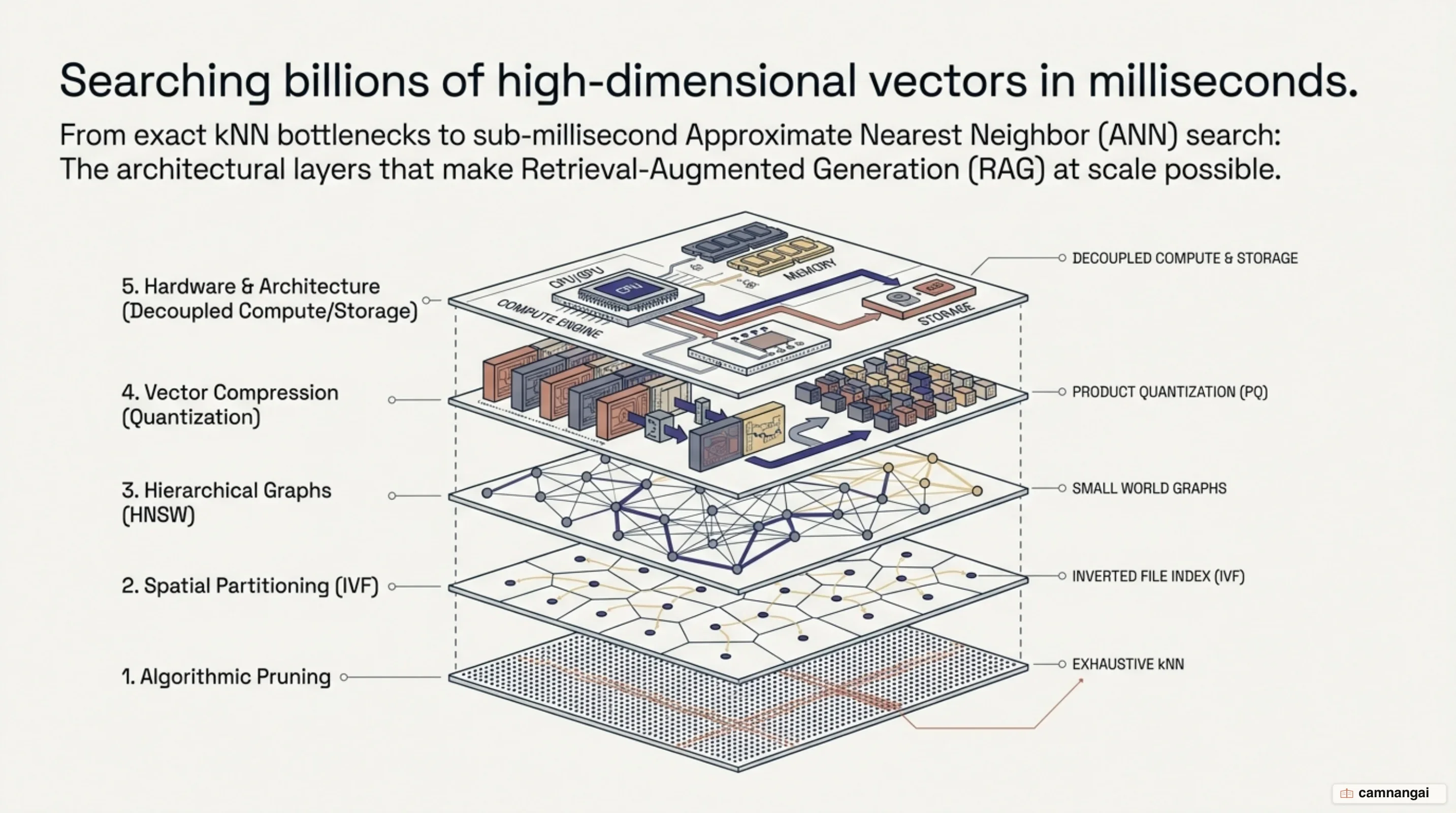
A vector database searches billions of high-dimensional vectors in milliseconds by replacing exhaustive brute-force calculations with Approximate Nearest Neighbor (ANN) indexing structures — specifically proximity graphs, space partitioning, vector quantization, and decoupled storage-compute architectures.
Instead of computing exact distances against every vector, these systems prune search spaces to logarithmic complexity, compress floating-point vectors by up to 97% or 40x, and offload full-precision rescoring to NVMe SSDs or blob storage.
To achieve sub-second query latency at billion scale, you must balance three competing variables: recall accuracy, query throughput (QPS), and memory consumption (RAM). Exhaustive linear search guarantees 100% recall but collapses under computational weight as datasets grow beyond millions of records. High-scale architectures resolve this by layering structural graph routing (such as HNSW) with aggressive lossy compression (Product, Scalar, or Binary Quantization) and disk-backed vector storage.
Understanding how these algorithms work beneath the software abstractions allows you to select the precise indexing parameters, hardware tiers, and filtering strategy for your specific operational workload.
Why brute-force search collapses at billion scale
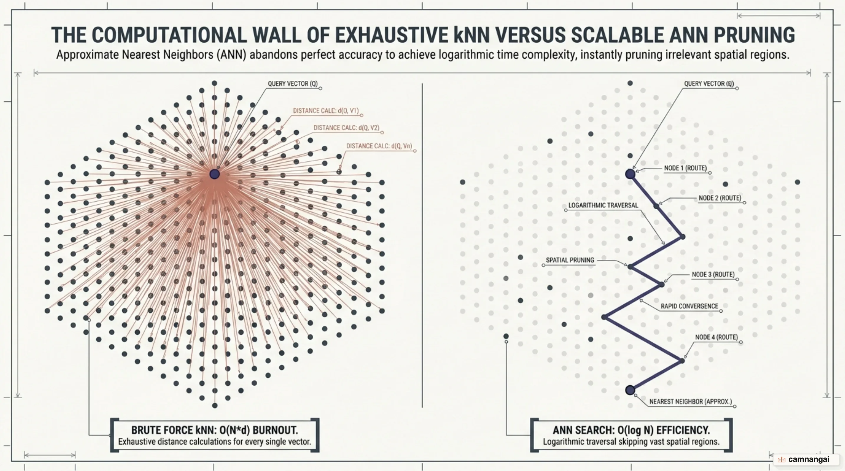
Exact k-nearest neighbor (kNN) search relies on uncompressed flat indexes, such as IndexFlatL2
(Euclidean distance) and IndexFlatIP (inner product/dot product). Flat indexes perform an unreduced
linear scan, comparing an incoming query vector xq against every single vector stored inside the
index across all D dimensions. Because no vector transformations, clustering, or graph shortcuts
are applied, flat indexes maintain 100% search quality and recall. However, this accuracy comes at the
cost of linear time complexity, denoted as O(N · D), where N is the total number of vectors and D
is the vector dimensionality.
Storing uncompressed floating-point vectors consumes substantial memory overhead. In standard vector
search implementations, vector dimensions are stored using single-precision floating-point numbers
(float32), where each scalar requires 4 bytes of storage. For a vector of dimension D, the raw
vector payload size is D * 4 bytes. Consequently, a 512-dimensional vector requires 2 KB of
uncompressed storage, while a 1536-dimensional vector requires 6 KB. To estimate total memory
requirements—including internal indexing data structures and graph overhead—you use the formula:
Memory Size = 1.5 * Number of Vectors * Dimension * 4 bytesApplying this formula demonstrates how memory costs scale rapidly:
- 100,000 vectors at 1536 dimensions (e.g., OpenAI
text-embedding-ada-002):1.5 * 100,000 * 1536 * 4 bytes ≈ 921.6 MB - 1,000,000 vectors at 128 dimensions (e.g., SIFT1M dataset):
1.5 * 1,000,000 * 128 * 4 bytes ≈ 768 MB - 1,000,000,000 vectors at 1536 dimensions:
1.5 * 1,000,000,000 * 1536 * 4 bytes ≈ 9.2 TB
Scaling an uncompressed in-memory flat index to 1 billion 1536-dimensional vectors requires over 9 TB of fast RAM solely to retain the index, making flat in-memory indexing economically and physically impractical for production systems.
Computational processing times collapse similarly under linear scaling. On a standard multi-core CPU running a flat L2 or IP index over a 1-million vector dataset (SIFT1M, 128 dimensions), a single query takes approximately 18 ms. When you scale the index size linearly to 1 billion vectors, single-query processing latency grows directly by 1,000x, requiring tens to hundreds of seconds per query. Production systems operating under real-time requirements cannot sustain exhaustive linear scans.
Space partitioning with IVF: Clustering to prune search spaces
The Inverted File Index (IVF) accelerates vector search by pruning the search space through geometric
partitioning, specifically Dirichlet tessellation (Voronoi space partitioning). Instead of evaluating
all N high-dimensional vectors, the database partitions the vector space into nlist distinct
Voronoi cells. Each cell is defined by a cluster centroid calculated by running k-means clustering
across the vector dataset during an explicit index training phase.
Voronoi Cell Construction (Space Partitioning):
+-------------------+-------------------+
|  .  * Centroid 1  |   .    .   .      |
| .   .    .        |  .  * Centroid 2  |
|    .    Cell 1    |   .    Cell 2     |
+-------------------+-------------------+
|   .   .           | .   .    .        |
|  .  * Centroid 3  |   . * Centroid 4  |
|    Cell 3         |   .    Cell 4     |
+-------------------+-------------------+
When you query an IndexIVFFlat structure, query execution follows a two-stage process:
- Centroid Lookup: Your engine calculates the distance between query vector
xqand allnlistcentroid vectors to identify the nearest Voronoi cells. - Cell-Restricted Search: Your engine restricts exhaustive distance evaluations exclusively to the vectors assigned to those selected Voronoi cells, completely bypassing the remaining partition cells across the database.
IVF Query Mechanics:
Query Vector (xq) ---> Compare with nlist Centroids
                           |
                           v
              Identify Nearest Cell Centroid(s)
                           |
                           v
        Scan Vectors ONLY inside matching Cell(s)
Partitioning space introduces the "edge problem." When your query vector xq lies near the boundary
of its enclosing Voronoi cell, its true nearest neighbor vectors may reside just across the boundary
inside an adjacent cell. If your search is limited strictly to the query vector's primary cell, those
true neighbors are omitted, causing recall to drop.
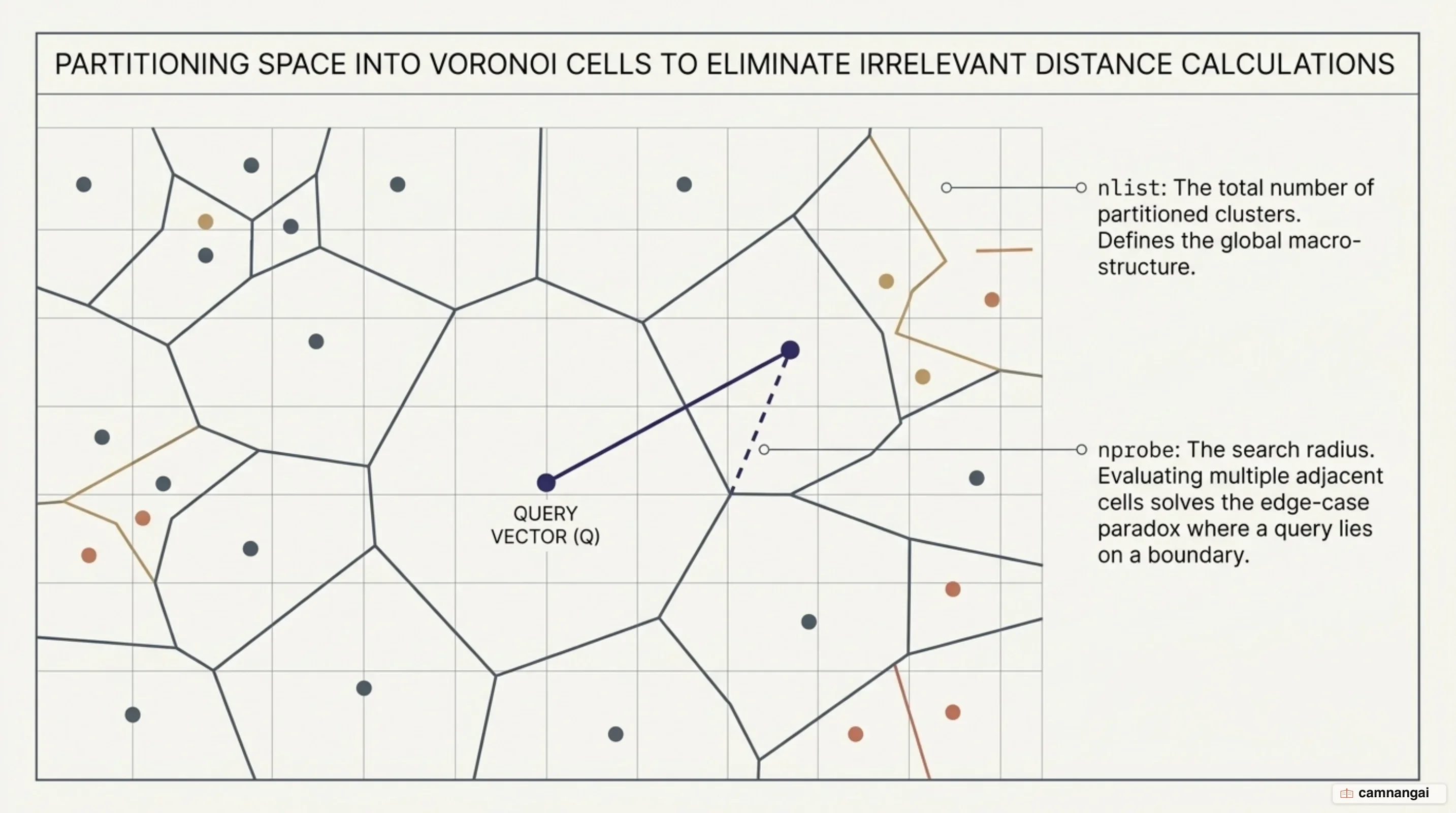
To resolve the edge problem, IVF exposes the nprobe query-time parameter, which dictates how many
adjacent Voronoi cells you inspect during a lookup. You must manage two primary configuration
trade-offs in IVF indexes:
nlist(Number of cells): Increasingnlistcreates finer partitions with fewer vectors per cell. This reduces the number of vector distance calculations per cell and speeds up search times, but requires more distance comparisons against cell centroids during initial routing.nprobe(Number of cells to search): Increasingnprobeexpands your query scope across multiple cell boundaries, directly improving recall accuracy at the cost of higher query latency.
HNSW graphs: Multi-layer expressways in high-dimensional space
Hierarchical Navigable Small World (HNSW) graphs adapt concepts from William Pugh's Probability Skip
Lists and Navigable Small World (NSW) proximity graphs to high-dimensional vector spaces. Standard NSW
graphs link vertices based on Euclidean proximity, maintaining a short average path length ("small
world" property) that yields logarithmic hop complexity O(log N) across connected networks.
However, standard NSW graphs suffer from premature convergence: search begins in low-degree nodes where greedy routing frequently gets trapped in local minima during its initial "zoom-out" routing phase. HNSW explicitly overcomes this structural flaw by reversing the entry topology. By placing high-degree, long-range link edges at the top of a multi-layer graph, HNSW forces your query to enter immediately into a "zoom-in" phase, routing rapidly across vast regions of the vector space before stepping down into denser lower layers.
HNSW Multi-Layer Expressway Topology:

Layer 2 (Sparse, Long-Range Edges):
Entry Point ---> [ Node A ] --------------------------> [ Node B ]
                     |                                      |
                     v                                      v
Layer 1 (Denser, Medium-Range Edges):
                 [ Node A ] --------> [ Node C ] ------> [ Node B ]
                     |                    |                 |
                     v                    v                 v
Layer 0 (Dense, Short-Range Edges - All Vectors):
                 [ Node A ] -> [ D ] -> [ C ] -> [ E ] -> [ B ]
HNSW structures these routing paths into a hierarchical multi-layer graph:
- Top Layers: Contain sparse nodes connected by long-range links. These top layers act as fast expressways for rapid coarse-grained routing across vast regions of the vector space.
- Lower Layers: Contain progressively denser nodes connected by shorter edges.
- Layer 0: The bottom layer contains every vector in the dataset connected via dense, short-range links for fine-grained local search.
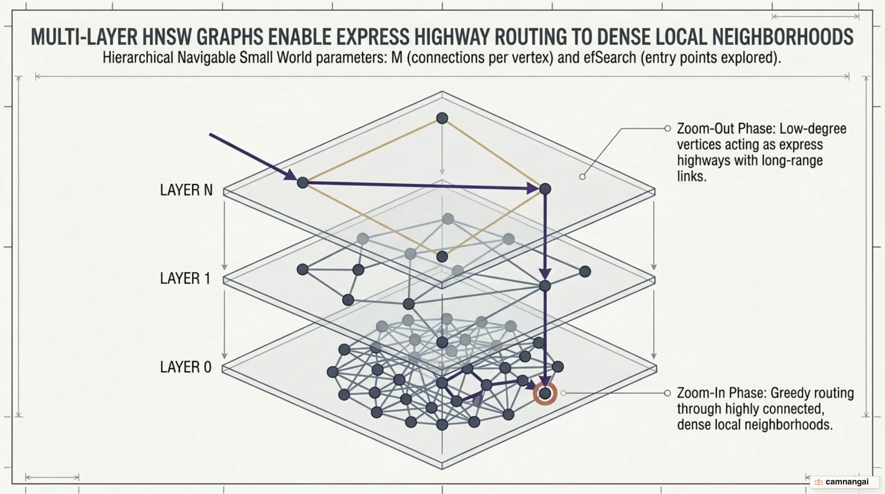
Query navigation begins at a designated entry point in the topmost layer. Your search algorithm
greedily traverses long-range edges to find the local minimum closest to query vector xq. Upon
reaching a local minimum at a given layer, the search drops down to the corresponding node in the layer
directly beneath it and resumes greedy traversal. This process repeats until reaching Layer 0, where
local searches refine candidate vectors to produce the final result set.
The trade-off of HNSW is its substantial memory overhead. A graph index with M = 64 edges per node
requires dozens of bytes of pointer metadata per vector, making pure in-memory billion-scale HNSW
prohibitively expensive without quantization.
Vector quantization: Fitting terabytes of data into RAM
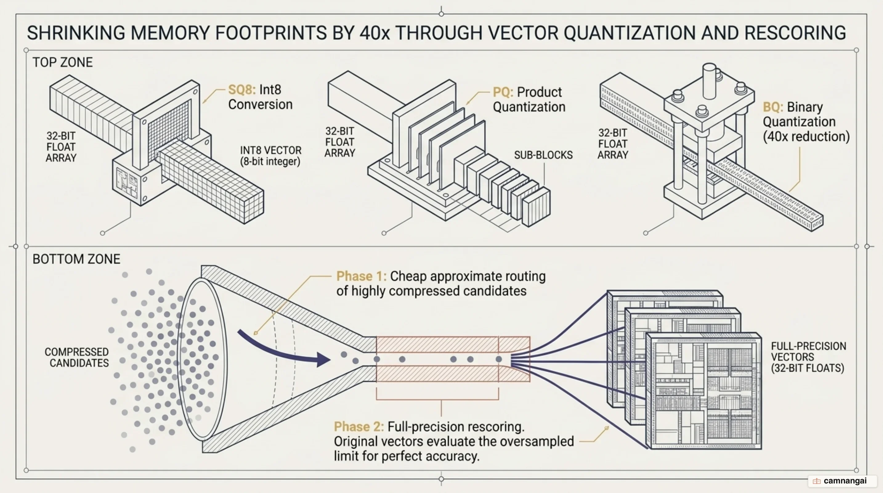
Vector quantization is a lossy compression technique that reduces the bit-depth of vector representations instead of reducing the number of dimensions. The primary quantization strategies in production vector databases are Scalar Quantization (SQ), Product Quantization (PQ), and Binary Quantization (BQ).
Scalar Quantization (SQ8) converts each 32-bit floating-point value (float32, 4 bytes) into an 8-bit
integer (int8, 1 byte), achieving an immediate 75% reduction in memory consumption. The linear
transformation maps values using scale (alpha) and offset constants:
f32 = alpha * i8 + offsetTo prevent distortion from extreme outliers, implementations apply quantile bounds (typically 0.95 to
0.99). Because offset and alpha factors can be precomputed, distance operations execute using
hardware-accelerated SIMD instructions (such as AVX-512 or ARM NEON), delivering 40–60% reductions in
query latency with less than 0.5% degradation in recall.
For higher scale, Product Quantization (PQ) and Binary Quantization (BQ) deliver deeper compression:
- Product Quantization (PQ): Decomposes a
D-dimensional vector intomlow-dimensional sub-vectors. The algorithm clusters each sub-space independently using k-means to generate a codebook of centroids. Each original sub-vector is then replaced with the 1-byte index of its nearest centroid. PQ compresses datasets by up to 97% (e.g., reducing 1 million 128-dimensional vectors from 256 MB to under 10 MB in IVFPQ indexes). - Binary Quantization (BQ): Compresses each floating-point dimension to a single bit (1 if greater
than 0, else 0). Taking advantage of the over-parameterization of large embedding models (1024 dimensions or
higher), BQ achieves up to 40x memory compression. Distance calculations collapse into bitwise XOR
operations combined with hardware
POPCNT(population count) instructions, increasing comparison speeds by up to 40x.
To recover accuracy, production systems deploy a two-phase Oversampling and Rescoring pipeline. In
phase one, the system uses the quantized in-memory index to retrieve an expanded candidate list
(top-(k * oversampling) with oversampling >= 2.0). In phase two, the engine fetches the original
full-precision float32 vectors from secondary storage (NVMe SSD) and recalculates exact similarity
scores, restoring high recall while keeping RAM usage minimal.
DiskANN and Vamana: Breaking the memory barrier with NVMe SSDs
When datasets expand past 1 billion vectors, total vector payloads and index structures require multiple terabytes of capacity. Keeping an entire graph index resident in RAM becomes cost-prohibitive.
DiskANN resolves this memory wall by constructing a flat Vamana graph designed specifically to live on NVMe SSD storage. The architecture separates routing from precision verification:
- Highly compressed vectors (quantized via PQ or SQ) remain in RAM to guide fast graph routing and candidate traversal.
- The complete uncompressed
float32vectors and the full Vamana adjacency lists reside directly on NVMe SSDs.
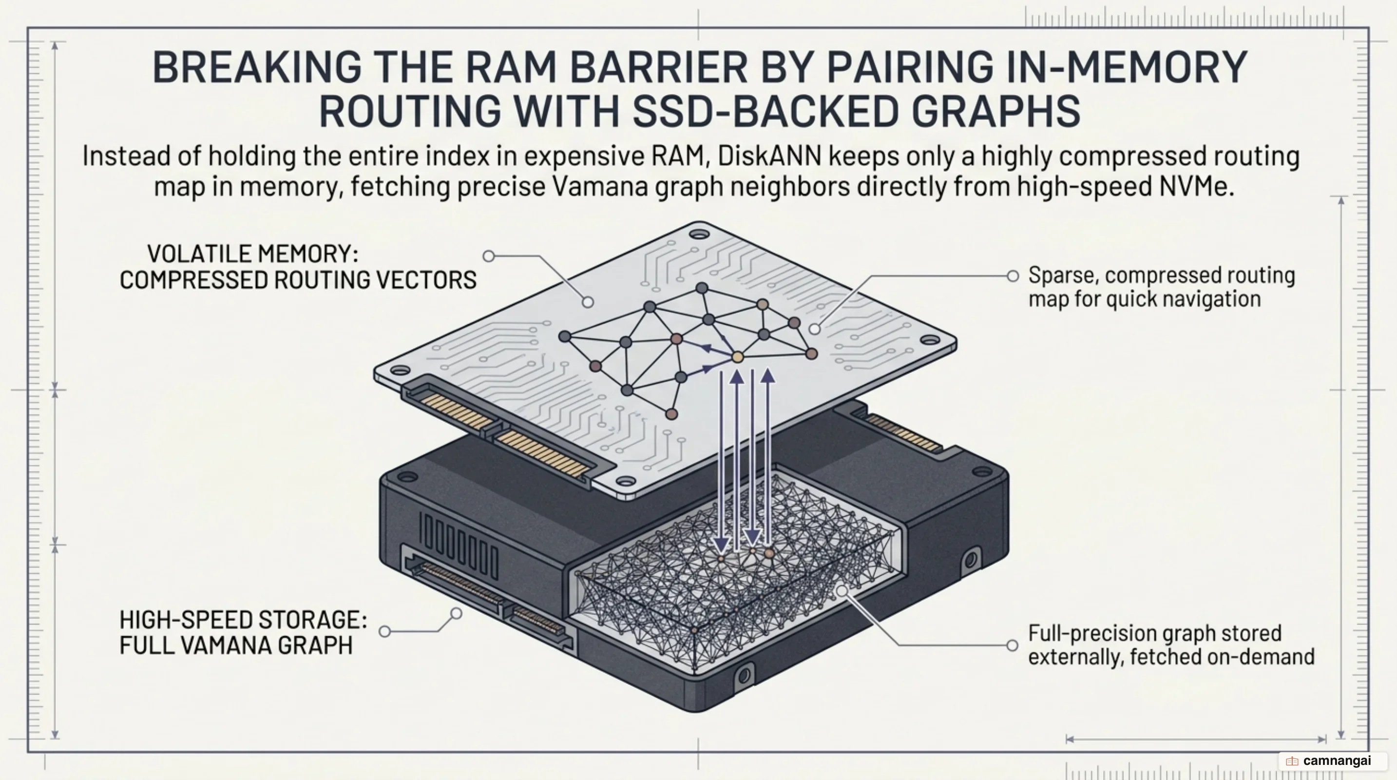
DiskANN takes advantage of the massive parallel random read throughput (IOPS) of modern NVMe drives. During graph traversal, the engine issues concurrent asynchronous I/O requests. By batching neighbor lookups across multiple frontier nodes in parallel, the algorithm minimizes sequential disk wait states during query routing.
Benchmark results show that DiskANN enables single-node billion-scale search on a machine with only 64 GB of RAM paired with commodity NVMe SSDs. It sustains thousands of queries per second (QPS) with over 95% recall and single-digit millisecond latency.
Real-time metadata filtering: Solving the pre vs post-filtering paradox
In real-world applications, vector similarity queries rarely run in isolation; they are accompanied by
metadata predicates—such as department == 'engineering' or created_at >= 2024. This introduces
"The Filter Problem" that causes traditional approaches to fail:
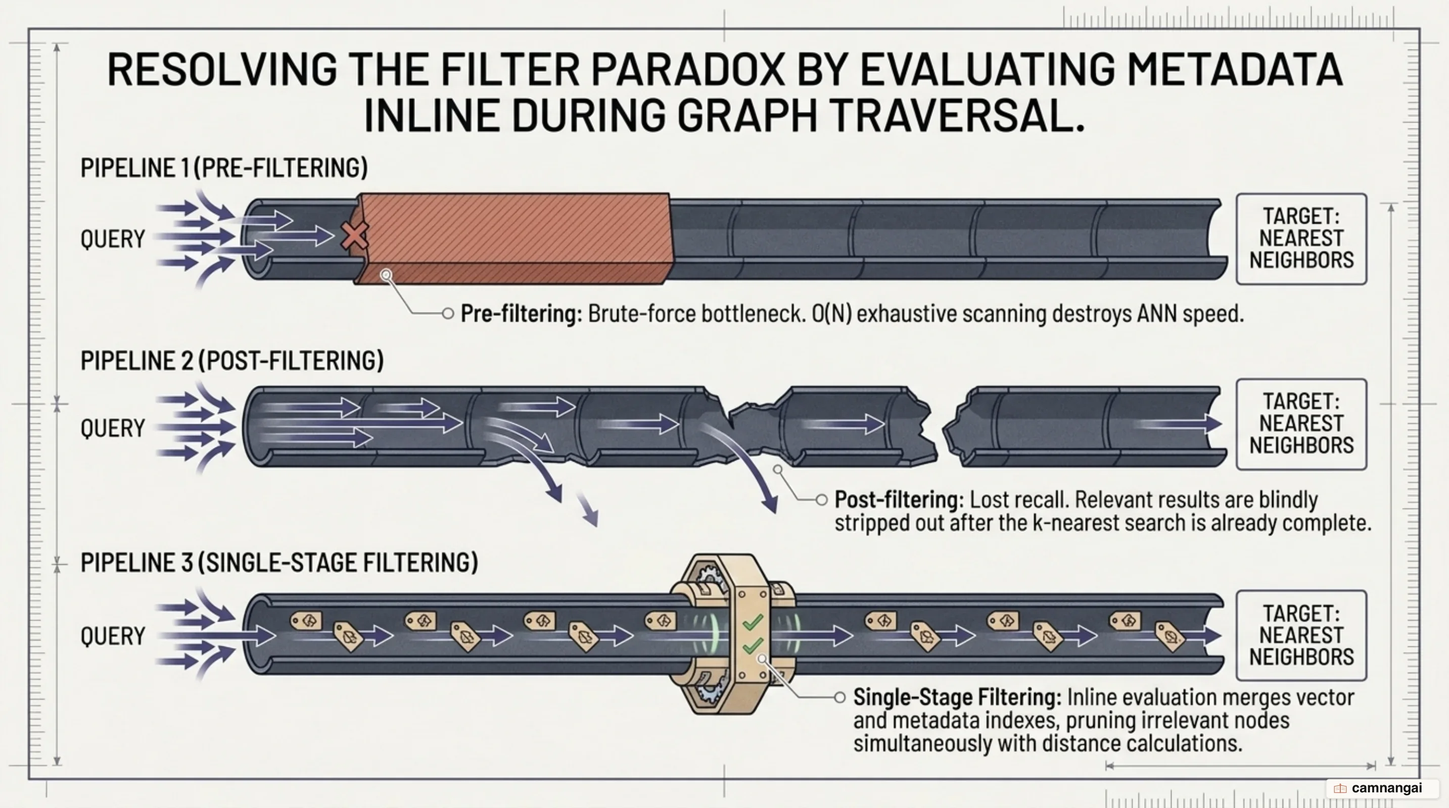
- Pre-filtering: Filtering metadata first generates an isolated ID allowlist, followed by vector search. Pruning nodes from the index before traversal breaks graph connectivity in algorithms like HNSW, forcing engines to fall back to slow linear scans across the matching subset.
- Post-filtering: Running vector search first to gather
top-kcandidates and applying metadata filters afterward risks returning fewer thankresults (or even zero results) if initial candidates fail the predicate filter.
Modern vector databases solve this with Single-Stage Filtering (implemented in engines like Pinecone and Milvus). This architecture fuses metadata attributes and vector graphs into a single unified indexing structure:
Single-Stage Filtering Architecture:
Query Vector + Metadata Filter Constraints
                    |
                    v
    +------------------------------------+
    | Integrated Graph & Metadata Index  |
    +------------------------------------+
                    |
        Evaluates metadata predicates
        concurrently during graph routing
                    |
                    v
  Prunes candidate score, preserves edge path
During graph traversal, the engine inspects metadata attributes directly on each candidate node. If a node fails the metadata predicate, the engine excludes it from the final candidate set but continues traversing its outbound edges to explore valid neighboring paths.
Empirical testing demonstrates that single-stage filtering maintains high recall while improving query latencies: queries with highly selective filters (matching 1% to 5% of data) execute faster than unfiltered queries because invalid branches are pruned early in the graph traversal.
Distributed architecture: Decoupling storage and compute in production
Monolithic or pod-based architectures face operational bottlenecks when scaling to billions of vectors under variable production traffic. Scaling compute requires over-provisioning memory, and handling traffic spikes often requires replicating entire multi-terabyte indexes.
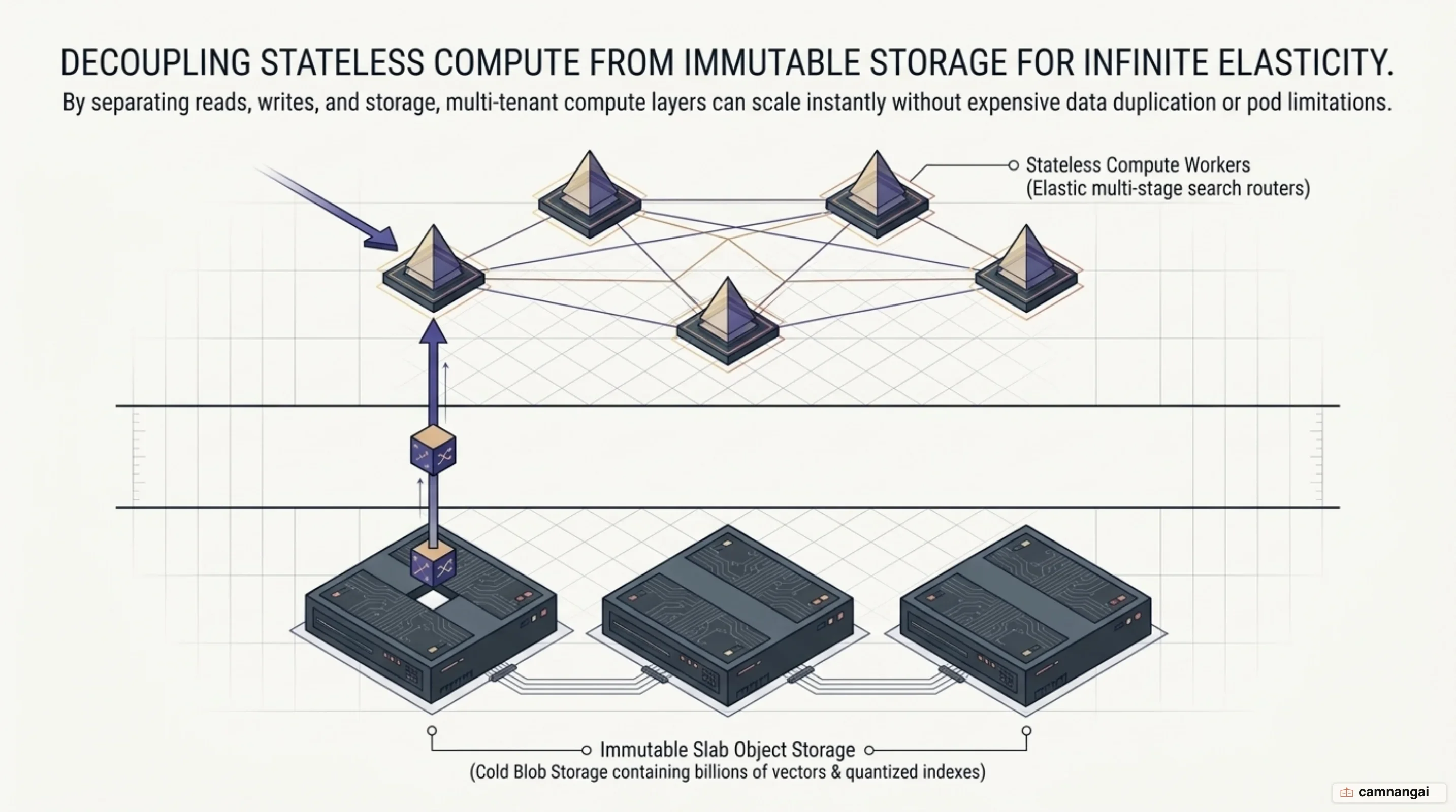
To overcome this, cloud-native vector databases adopt a decoupled storage and compute architecture. The system separates operational responsibilities into three independent tiers:
Decoupled Serverless Architecture:
                +----------------------------+
                | Stateless Worker Nodes     |
                | (Query Execution & Reads)  |
                +----------------------------+
                   /                       \
        Read Queries /                      \ Data Ingestion /
        Local Cache                          \ Index Building
                 v                           v
     +---------------------------------------------------+
     | Centralized Object Storage (e.g. S3 / GCS)        |
     | (Space-Clustered Immutable Slabs)                 |
     +---------------------------------------------------+
Key operational principles of this architecture include:
- Immutable Slabs in Object Storage: Vector embeddings and index partitions are organized into space-clustered, immutable data files (slabs) persisted in low-cost object storage.
- Stateless Compute Workers: Query nodes execute distance comparisons and graph routing without maintaining permanent local state, allowing workers to scale horizontally based on query demand.
- Intelligent Local Caching: Query nodes download and cache index centroids and active segment namespaces on local NVMe caches for frequently queried ("warm") datasets, eliminating network storage penalties for active workloads.
This decoupled architecture allows compute capacity to scale dynamically with query throughput while storage scales independently with vector volume. Organizations eliminate idle hardware costs while confidently serving billion-scale workloads.
Choosing the right vector indexing architecture for your workload
Selecting the appropriate vector indexing strategy requires balancing dataset scale, query latency targets, and infrastructure budget:
| Dataset Scale | Primary Constraint | Recommended Architecture |
|---|---|---|
| Below 10,000 vectors | 100% precision required | Flat (IndexFlatL2 / IndexFlatIP), no indexing required |
| Below 10 million vectors | Sub-2ms latency, 95–100% recall | Pure in-memory HNSW (unconstrained RAM) |
| 10M to 100M+ vectors | Memory-efficient single server | HNSW with SQ8, or IVF-PQ with oversampling |
| Over 1 billion vectors | Constrained RAM, cost-sensitive | DiskANN (Vamana on NVMe SSD) + Oversampling & Rescoring |
| Multi-tenant variable traffic | Minimal ops, elastic autoscaling | Cloud-native Serverless (Decoupled Blob Storage + Stateless Compute) |
Approximate Nearest Neighbor Search (ANNS) in vector databases is always an engineering trade-off between latency, recall, and infrastructure cost. Understanding the mechanics of HNSW, IVF, quantization, and disk-backed graphs ensures you build resilient retrieval infrastructure tailored to your AI applications.
References
- Faiss: A library for efficient similarity search — Engineering at Meta
- Hierarchical Navigable Small Worlds (HNSW) — Pinecone
- Nearest Neighbor Indexes for Similarity Search — Pinecone
- Product Quantization: Compressing high-dimensional vectors by 97% — Pinecone
- Scalar Quantization for Vector Search — Qdrant
- Binary Quantization: 40x Faster Vector Search — Qdrant
- Disk-based DiskANN: High Recall and QPS on Billion-scale Datasets — Zilliz blog
- The Missing WHERE Clause in Vector Search — Pinecone
- Introducing Pinecone Serverless — Pinecone