Data Classification with Embeddings: From Vectors to Categories

Data classification with embeddings is the process of converting unstructured text into dense numerical vectors and using those vectors as feature inputs for a supervised learning algorithm.

This approach allows you to categorize information based on semantic meaning rather than relying on exact word overlaps or syntax.

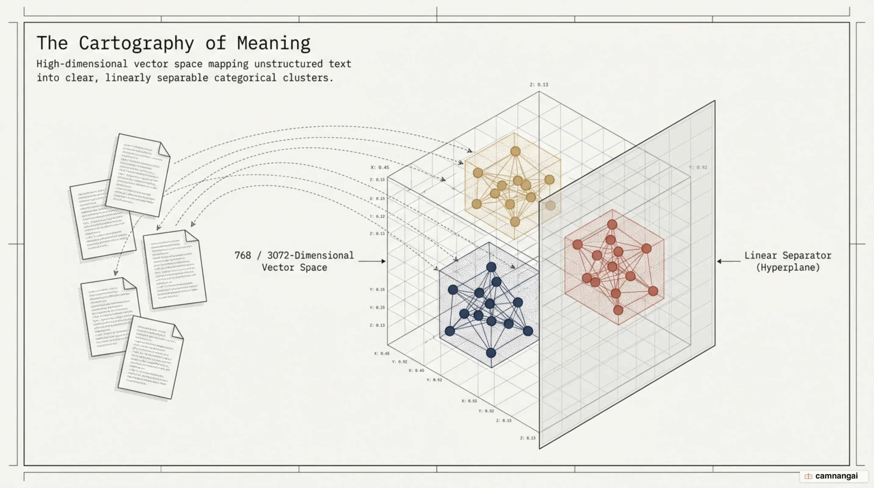
By representing text in a high-dimensional vector space, you enable your system to recognize that different words can describe the same underlying concept. You map arbitrary-length text into a structured format that standard estimators process with high precision. This method is effective when you have a fixed set of categories and enough labeled data to satisfy the computational requirements of high-dimensional feature matrices.

In an engineering context, this pipeline replaces sparse, high-cardinality features with dense representations that capture latent relationships. Using this technique, you can build classifiers that understand the intent of a passage, delivering a reliable solution for tasks ranging from sentiment analysis to automated fraud detection.

Data classification with embeddings in high-dimensional vector space

How embedding-based data classification works

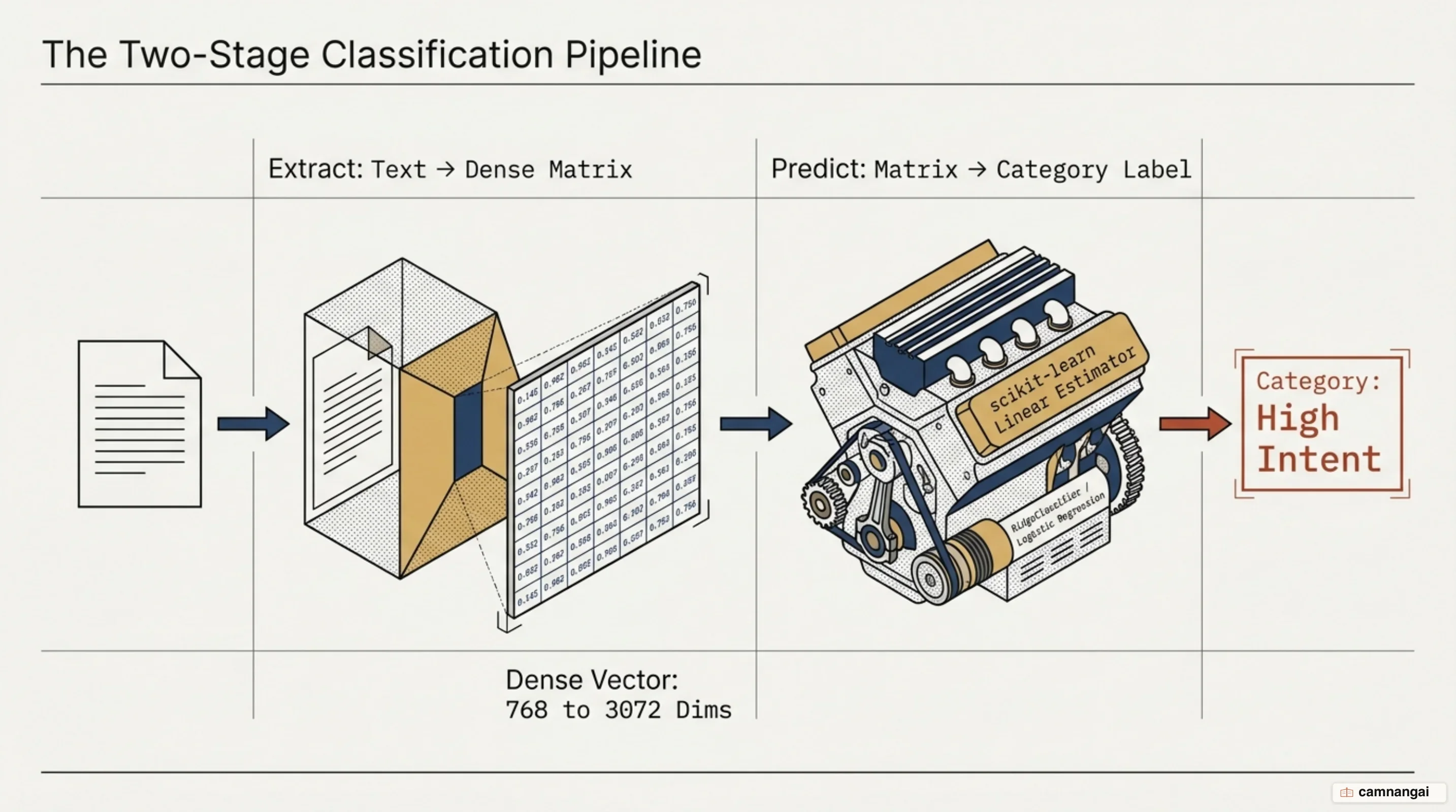
The technical pipeline for data classification with embeddings consists of two distinct stages. First, raw text is processed through a pre-trained embedding model, such as gemini-embedding-001. This model transforms the text into a dense vector representation. These vectors are typically high-dimensional; while some models produce 768 dimensions, gemini-embedding-001 generates 3072-dimensional vectors.

Unlike sparse vectors (such as one-hot encodings), which map specific words to indices, these dense vectors represent meaning through deep-learning methods similar to those used in large language models. In the second stage, these vectors serve as the feature matrix ($X$) for a traditional supervised learning estimator. The estimator is trained on labeled data to learn a mapping between these high-dimensional points in the vector space and specific categorical labels ($y$).

Two-stage data classification pipeline from dense embedding model to supervised estimator

Why embeddings outperform traditional classification features

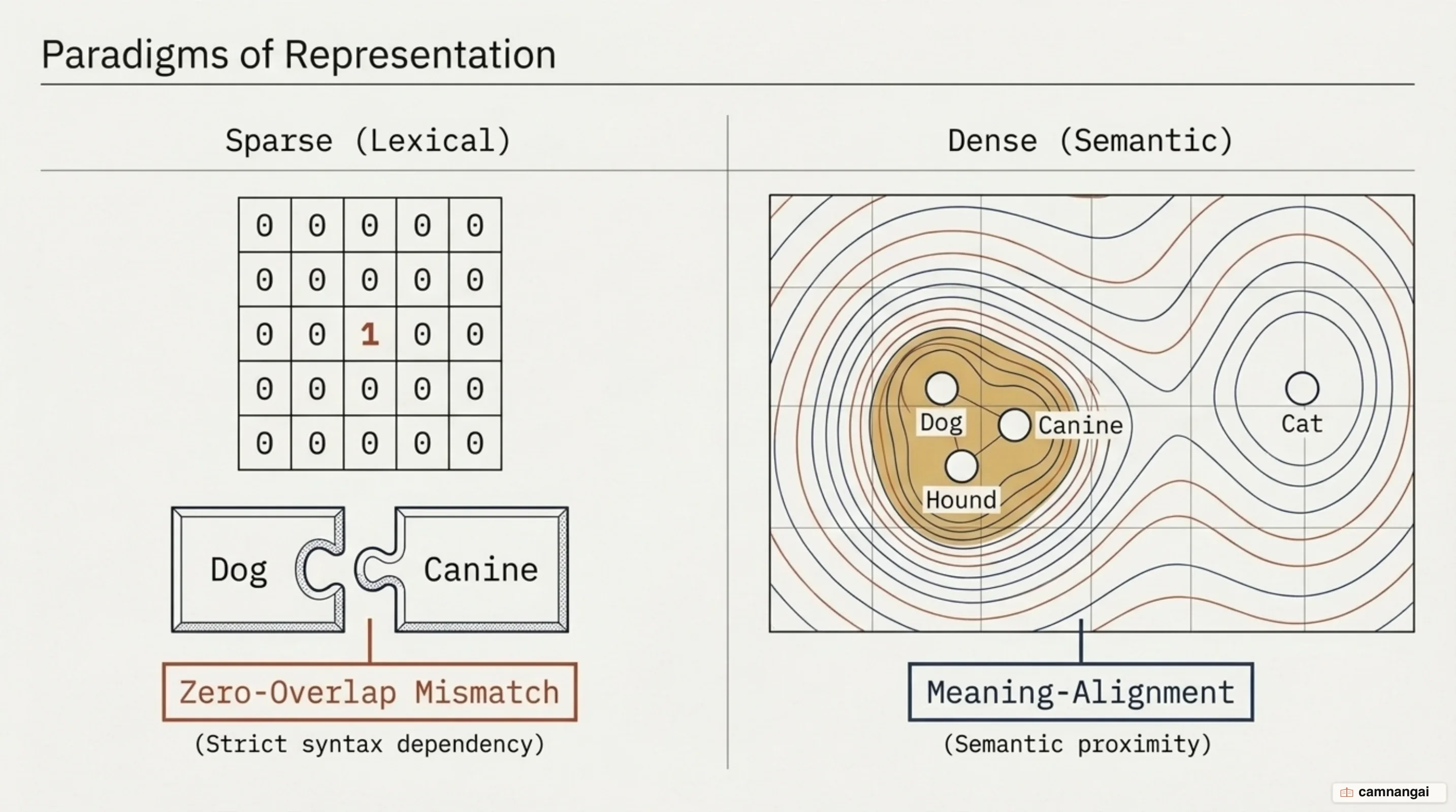
Dense embeddings offer significant advantages over traditional sparse vectors like frequency counts. Sparse vectors rely on direct word or syntax matches, which frequently fail when the same concept is described using different vocabulary. Embeddings solve this through meaning-alignment, allowing a classifier to correctly identify a relevant passage even if it shares zero keywords with the training examples, provided their semantic vectors are proximal in the vector space.

Comparison between traditional sparse keyword vectors and dense semantic embeddings

On top of that, embeddings provide a practical form of efficiency and compression. While models generate full-length vectors by default (e.g., 3072 dimensions), you can use parameters like output_dimensionality to truncate the vector size. This reduction saves significant storage and compute resources for downstream applications while incurring a minimal loss in output quality.

Core classification algorithms trained on vector embeddings

Several linear models and ensemble methods are particularly effective when using embeddings as features:

Logistic Regression: Often referred to as a log-linear classifier, this model handles binary, One-vs-Rest, or multinomial problems. For numerical stability, the "lbfgs" solver is the default. For smaller datasets, "liblinear" is efficient, while the "saga" solver is optimized for large-scale multinomial problems but requires scaled data for convergence.
Ridge Classifier: This variant converts binary targets to -1 and +1 and treats classification as a regression task (multi-output regression for multiclass). It is significantly faster than Logistic Regression for high class counts because it can compute the projection matrix $(X^T X)^-1 X^T$ only once and reuse it across outputs.
Random Forest: This ensemble method is a practical choice for handling the inherent subjectivity in human-labeled data, such as 1–5 star food reviews. It is effective at distinguishing categories even when the boundaries between classes (like a 2-star vs. 3-star review) are subtle.

The following scikit-learn example demonstrates a basic fit using a Ridge classifier:

python

from sklearn.linear_model import RidgeClassifier
 
# X_train: np.ndarray of shape (n_samples, n_features)
# y_train: np.ndarray of shape (n_samples,)
# Note: For gemini-embedding-001, n_features = 3072
clf = RidgeClassifier(alpha=1.0)
clf.fit(X_train, y_train)
 
# Predict categories for new embeddings
predictions = clf.predict(X_test)

Architecture trade-offs: Embeddings + Classifier vs Fine-tuning vs Prompting

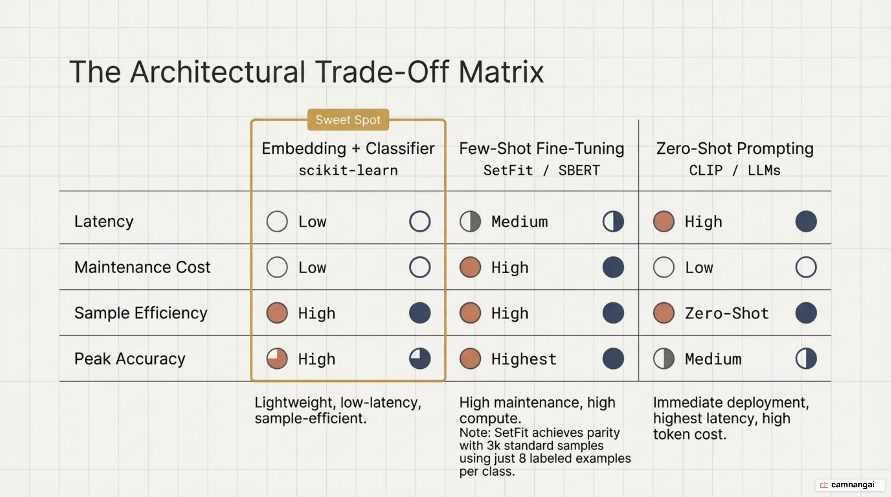
While fine-tuning a full model may offer higher accuracy for specific niche tasks, the Embedding + Classifier approach is often more computationally accessible and easier to deploy in production.

Architecture trade-off comparison between Embedding + Classifier, Fine-tuning, and Zero-shot Prompting

One hard engineering constraint is the examples-to-dimensions rule: to avoid the curse of dimensionality and overfitting, you generally need a training dataset where the number of samples significantly exceeds the number of embedding dimensions. For example, using gemini-embedding-001 with 3072 dimensions requires a much larger labeled dataset to reach stability compared to a 768-dimensional model. In cases where the number of samples is small relative to the feature count, the model is likely to overfit the noise in the high-dimensional space.

Computational complexity is another factor. For algorithms like Ordinary Least Squares or Ridge, the training cost scales quadratically with dimensionality, approximately $O(N \cdot D^2)$ where $N$ is sample count and $D$ is feature dimensions. This quadratic dependence on the number of features highlights the importance of choosing an appropriate embedding dimension; reducing a vector from 3072 to 768 dimensions can result in a 16x speedup in the classifier training phase.

Real-world applications and common engineering pitfalls

Embedding-based classification is widely used across several domains:

News Classification: Categorizing articles into fixed bins such as Business, Politics, or Entertainment.
Sentiment Analysis: Predicting scores (e.g., 1–5 stars) in food or product reviews.
Fraud Detection: Modeling the probability of a fraudulent financial transaction as a Bernoulli trial.

A common engineering pitfall is class imbalance. In a 1–5 star review dataset, 5-star reviews are often over-represented. This leads to high precision for the majority class but poor recall for minority classes (1–2 stars), as the model has fewer examples of negative sentiment to learn from.

Another key requirement is handling unscaled data. The feature matrix ($X$) should be standardized before fitting. While solvers like "lbfgs" tolerate unscaled datasets better, solvers like "saga" require scaling for convergence. Also, when applying L2 regularization (as in Ridge or Logistic Regression), standardization is non-negotiable to ensure the penalty treats all dimensions equally, preventing features with larger magnitudes from disproportionately influencing the model.

When to use embedding-based classification in production

The engineering verdict for this approach is positive when you have a fixed set of categories and a labeled dataset that is larger than the dimensionality of your embeddings. This method provides a stable, high-performance alternative to the latency and cost of prompting LLMs for every classification request.

If your training labels are corrupted by significant outliers or high human subjectivity, you should pivot from standard linear models to outlier-resistant estimators. Models such as RANSAC or the Huber Regressor can be used to minimize the impact of outlying data points, ensuring the classifier remains aligned with the primary data distribution.