What is an Attention Mechanism? How Neural Networks Learn to Focus

In deep neural networks, an attention mechanism is a computational module that calculates a vector of dynamic importance weights over input representations, allowing your network to focus on specific parts of a sequence regardless of distance.

When you process sequential data, rather than compressing an entire input sequence into a single static embedding, an attention mechanism evaluates the relative relevance of every source token when generating or transforming a given target token.

When you trace the evolution of sequence models, early sequence-to-sequence architectures relied on recurrent neural networks that squeezed variable-length inputs into fixed-length context vectors. This architectural pattern created a severe information bottleneck that degraded performance on long sequences through signal decay and catastrophic forgetting. The introduction of attention mechanisms replaced these static representations with dynamically weighted sums over encoder hidden states, creating direct, content-addressable shortcut connections across sequence positions.

By routing information dynamically based on key-query alignment, you eliminate the information loss inherent in fixed-length vector bottlenecks and enable complete intra-example parallelization across sequence positions.

This structural shift overcomes the primary hardware execution constraints of recurrent architectures and forms the core foundation of modern Transformer models.

The Seq2Seq Bottleneck and Why Attention Was Invented

When you design classical sequence transduction models using recurrent encoder-decoder frameworks (Sutskever et al., 2014), your architecture transforms an input sequence (x_1, x_2, ..., x_n) into a target sequence (y_1, y_2, ..., y_m) of arbitrary length. In these traditional systems, an encoder built from recurrent neural network (RNN) layers—such as Long Short-Term Memory (LSTM) or Gated Recurrent Unit (GRU) networks—processes source tokens sequentially. To capture context from both directions, you typically employ a bidirectional RNN where forward and backward hidden states are concatenated to form a composite annotation. The encoder compresses this entire sequence into a single fixed-length context vector c, passing it to the decoder as the initial hidden state s_0.

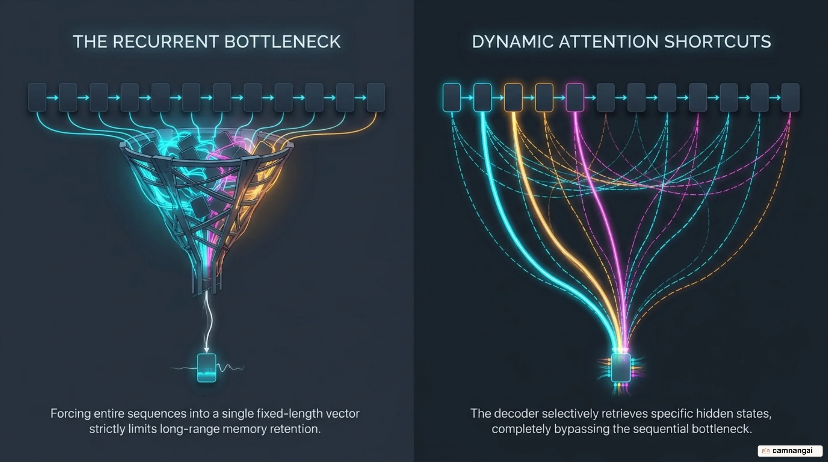
This reliance on a single fixed-length context vector introduces a severe mathematical bottleneck into your pipeline. Because the context vector c has a fixed dimensionality d_model, its total information capacity is fixed regardless of whether your input sequence contains 5 tokens or 500 tokens. As your recurrent encoder iterates through step-by-step transformations (h_t = f(h_{t-1}, x_t)), early hidden states are repeatedly overwritten by subsequent linear algebra transformations and non-linear activations. As a result, when you process long sequences, the network forgets early source tokens by the time the encoder reaches the end of the input, causing severe translation and generation degradation.

From a hardware systems perspective, traditional recurrent models suffer from fundamental parallelization limits. Recurrent state calculations factor computation along the temporal time steps of input and output sequences. Because the calculation of state h_t strictly requires the prior state h_{t-1}, you cannot compute operations across sequence positions in parallel within a single training example. This sequential operational dependency restricts GPU Tensor Core throughput, inflates training wall-clock time, and limits your maximum minibatch size under fixed VRAM constraints.

Path length dynamics further compound the difficulty of learning long-range dependencies in recurrent layers. Signal forward-propagation and gradient back-propagation must traverse a sequence of operational steps that grows linearly O(n) with sequence length n. While alternative architectures like ConvS2S and ByteNet reduced maximum network path lengths to O(n/k) or O(log_k n) by stacking convolutional kernels of width k, they required multi-layered hierarchies to connect distant tokens. To resolve these bottlenecks simultaneously, Bahdanau et al. (2015) introduced direct shortcut connections between the decoder and all intermediate encoder hidden states. By calculating dynamically learned alignment weights alpha_{t,i}, your model constructs context vectors c_t = Σ (alpha_{t,i} · h_i) tailored specifically to each output step t, bypassing the fixed-length vector constraint entirely.

Mathematical Formulation: Queries, Keys, Values, and Scoring Functions

To engineer an attention mechanism, you can conceptualize it formally as a dynamic memory retrieval operation that maps a Query vector q and a set of Key-Value vector pairs (k_i, v_i) to an output vector. Given a query q, a matrix of n keys K, and a matrix of n values V, your attention layer calculates a vector of scalar alignment weights using a specialized scoring function. The module then computes its final output vector as a weighted sum over value vectors:

text

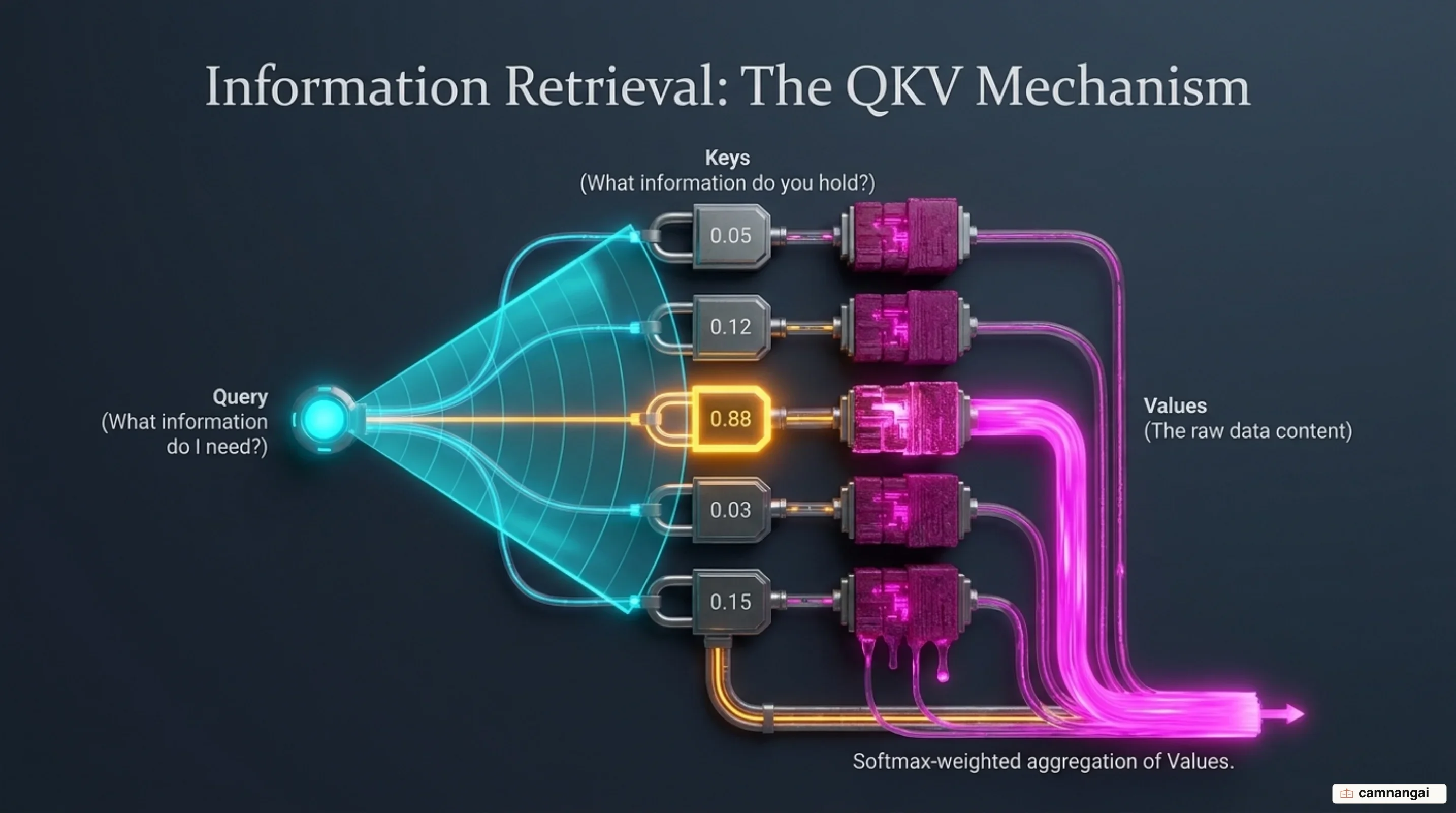
Output = Σ (α_i · v_i)

where each scalar weight alpha_i represents the normalized compatibility score between query q and key k_i.

The core behavior of your attention module depends on your choice of attention scoring function score(q, k_i). Additive Attention (Bahdanau et al., 2014) maps queries q and keys k into a shared hidden representation space of dimension h using learnable weight parameters W_q, W_k, and v_a. The formal scoring equation is defined as:

text

score(q, k) = v_a^T · tanh(W_q · q + W_k · k)

This structure functions identically to a single-hidden-layer feed-forward network using a tanh activation function without bias terms. The primary practical advantage of additive attention is its ability to handle queries and keys with unequal vector dimensions. However, executing additive attention incurs higher GPU memory overhead due to the explicit projection passes and activation steps involved.

Dot-Product Attention (Luong et al., 2015) replaces the feed-forward network with a simplified inner product operation. When query and key dimensions match, the scoring function is evaluated directly as score(s_t, h_i) = s_t^T · h_i. If vector dimensions differ, you can project them into alignment using a parameter matrix W_a, yielding score(s_t, h_i) = s_t^T · W_a · h_i. Dot-product attention is substantially faster and more space-efficient in production hardware deployments because it relies entirely on Level 3 BLAS Basic Linear Algebra Subprograms, mapping directly to high-throughput matrix multiplication operations on modern accelerators.

When you deploy attention modules on minibatches containing sequences of variable lengths, you must prevent zero-padded dummy tokens from corrupting your attention distributions and model gradients. You solve this through a Masked Softmax Operation. For any padded token position beyond the true sequence length l, you override its raw unnormalized logit score with a large negative value (such as -1e6 or -inf). The exponentiated values of masked positions evaluate to zero in softmax, guaranteeing that padded tokens receive exactly zero weight in downstream value aggregations and contribute zero gradient during backpropagation. To execute these operations concurrently across a batch of n sequences, you run Batch Matrix Multiplication (BMM) across 3D query and key batch tensors.

Scaled Dot-Product Attention: The Core Transformer Engine

When Vaswani et al. (2017) designed the Transformer architecture, they established Scaled Dot-Product Attention as its main computational engine. When you process a batch of queries packed into matrix Q, keys packed into matrix K, and values packed into matrix V, your layer executes attention simultaneously across all sequence positions using the matrix equation:

text

Attention(Q, K, V) = softmax((Q · K^T) / √d_k) · V

The intermediate matrix product Q · K^T evaluates pairwise unnormalized dot products between every query vector and every key vector across your input representations.

text

+-----------------------------------------------------------------------+
|                    SCALED DOT-PRODUCT ATTENTION                       |
|                                                                       |
|  Queries (Q) [n x d_k]  x  Keys (K^T) [d_k x m]                       |
|                             |                                         |
|                             v                                         |
|                   Raw Logits [n x m]                                  |
|                             |                                         |
|                             v                                         |
|              Scale by (1 / sqrt(d_k))  <-- Prevents Saturation       |
|                             |                                         |
|                             v                                         |
|              Apply Masked Softmax (valid_lens)                        |
|                             |                                         |
|                             v                                         |
|              Attention Weights (α) [n x m]                            |
|                             |                                         |
|                             v                                         |
|  Attention Weights [n x m]  x  Values (V) [m x d_v]                   |
|                             |                                         |
|                             v                                         |
|                  Output Tensor [n x d_v]                              |
+-----------------------------------------------------------------------+

The mathematical proof for scaling your dot products by 1 / √d_k centers on maintaining unit variance in your attention logits. Assume that the vector elements of query q and key k are independent random variables with a mean of 0 and a variance of 1. Their dot product is expressed as q · k = Σ (q_i · k_i). Because q_i and k_i are independent, the mean of their product is zero. The variance of the sum of d_k independent random variables each with variance 1 evaluates directly to d_k.

As your vector feature dimension d_k grows large, the standard deviation of raw dot products scales to √d_k. Large magnitude logits push your softmax activations into regions of extreme saturation where output gradients approach zero. By dividing Q · K^T by √d_k, you scale logit variance back down to 1, maintaining stable gradient flow during backpropagation.

To regularize your scaled dot-product attention module, you apply dropout directly to the computed attention weight matrix prior to multiplying by the value matrix V. Applying dropout randomly zeros out individual elements in the attention distribution matrix with probability P_drop and scales remaining weights by 1 / (1 - P_drop). This prevents your model from developing co-adapted parameter dependencies along specific query-key alignment paths during training.

Below, you can review a clean PyTorch implementation of Scaled Dot-Product Attention featuring masked softmax handling and dropout:

python

import math
import torch
import torch.nn as nn
 
def masked_softmax(X: torch.Tensor, valid_lens: torch.Tensor) -> torch.Tensor:
    """Perform softmax operation by masking elements along the last axis.
 
    Shapes:
        X: (batch_size, num_queries, num_keys)
        valid_lens: (batch_size,) or (batch_size, num_queries)
    """
    if valid_lens is None:
        return nn.functional.softmax(X, dim=-1)
 
    shape = X.shape
    if valid_lens.dim() == 1:
        valid_lens = torch.repeat_interleave(valid_lens, shape[1])
    else:
        valid_lens = valid_lens.reshape(-1)
 
    flat_X = X.reshape(-1, shape[-1])
    maxlen = flat_X.size(1)
    mask = torch.arange(maxlen, dtype=torch.float32, device=X.device)[None, :] < valid_lens[:, None]
 
    flat_X[~mask] = -1e6
    return nn.functional.softmax(flat_X.reshape(shape), dim=-1)
 
 
class DotProductAttention(nn.Module):
    """Scaled Dot-Product Attention engine with masked softmax regularization."""
    def __init__(self, dropout: float):
        super().__init__()
        self.dropout = nn.Dropout(dropout)
        self.attention_weights = None
 
    def forward(
        self,
        queries: torch.Tensor,
        keys: torch.Tensor,
        values: torch.Tensor,
        valid_lens: torch.Tensor = None
    ) -> torch.Tensor:
        """Executes forward pass over batch inputs.
 
        Shapes:
            queries: (batch_size, num_queries, d_k)
            keys:    (batch_size, num_keys, d_k)
            values:  (batch_size, num_keys, d_v)
            valid_lens: (batch_size,) or (batch_size, num_queries)
            Output:  (batch_size, num_queries, d_v)
        """
        d_k = queries.shape[-1]
        scores = torch.bmm(queries, keys.transpose(1, 2)) / math.sqrt(d_k)
        self.attention_weights = masked_softmax(scores, valid_lens)
        return torch.bmm(self.dropout(self.attention_weights), values)

Self-Attention vs. Cross-Attention: How Networks Relate Sequences

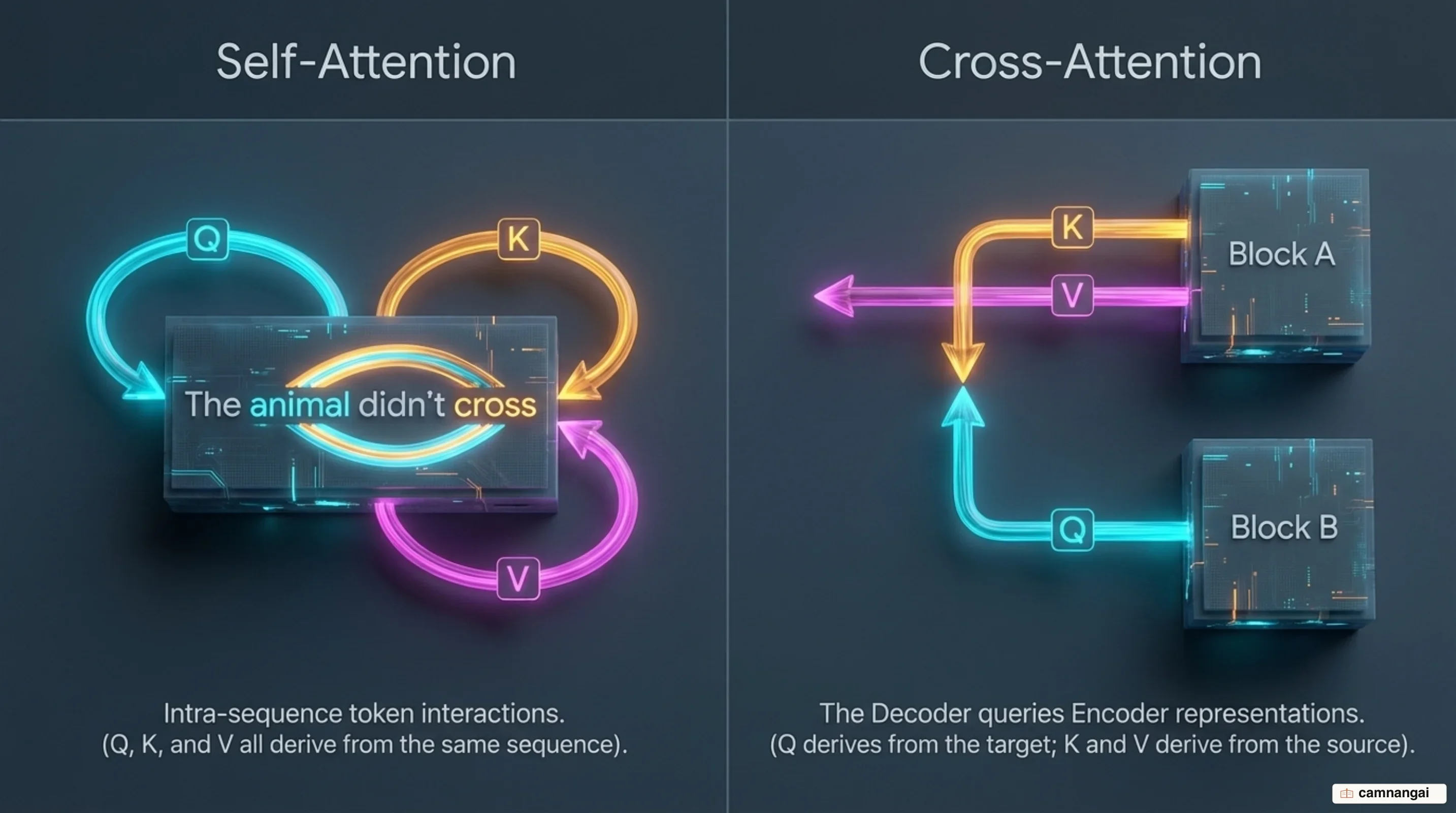
In transformer systems, Self-Attention describes an attention operation where your Queries, Keys, and Values all originate from the exact same sequence representation. Rather than calculating dependencies between disparate modalities or separate input-output sequences, self-attention maps an input sequence against itself. This allows each token in a sentence to attend to every other token in the same sentence, extracting deep syntactic dependencies and resolving co-referential references (such as mapping the pronoun "it" back to "the animal" in complex grammatical contexts).

text

+--------------------------------------------------------------------------+
|                  SELF-ATTENTION vs. CROSS-ATTENTION                      |
|                                                                          |
|  [ SELF-ATTENTION ]                                                      |
|                                                                          |
|  Input Sequence X  -----> Linear(W_Q) ------> Queries (Q)                |
|                    -----> Linear(W_K) ------> Keys (K)     ==> Attention |
|                    -----> Linear(W_V) ------> Values (V)                 |
|                                                                          |
|  * All Q, K, V derived from the same source sequence *                  |
|                                                                          |
|  [ CROSS-ATTENTION ]                                                     |
|                                                                          |
|  Decoder State S   -----> Linear(W_Q) ------> Queries (Q)                |
|                                                            ==> Attention |
|  Encoder Memory H  -----> Linear(W_K) ------> Keys (K)                   |
|                    -----> Linear(W_V) ------> Values (V)                 |
|                                                                          |
|  * Queries from decoder; Keys and Values from encoder memory *           |
+--------------------------------------------------------------------------+

In contrast, Cross-Attention (or encoder-decoder attention) pulls its input representations from two distinct sources. In sequence transduction pipelines, your Queries are projected from the current decoder hidden states, while your Keys and Values are projected from the final encoder output representations. In this topology, cross-attention acts as a dynamic retrieval bridge: each generating token in the decoder queries the complete, uncompressed contextual memory of the source sequence to determine which input features to integrate into the output representation.

When you implement self-attention inside the decoder of an autoregressive generative model (like GPT), you must strictly enforce Causal Masking (look-ahead masking). Because autoregressive generation requires that the prediction for token y_t depends solely on previously generated tokens, your attention layer must prevent future tokens from leaking into past representations. You implement causal masking by adding an upper-triangular mask matrix where entries above the main diagonal evaluate to -inf. When added to the raw logit scores before the softmax operation, future positions evaluate to zero probability, preserving the directional autoregressive factorization of your sequence probability distribution during both training and inference.

Multi-Head Attention: Attending to Multiple Representation Subspaces

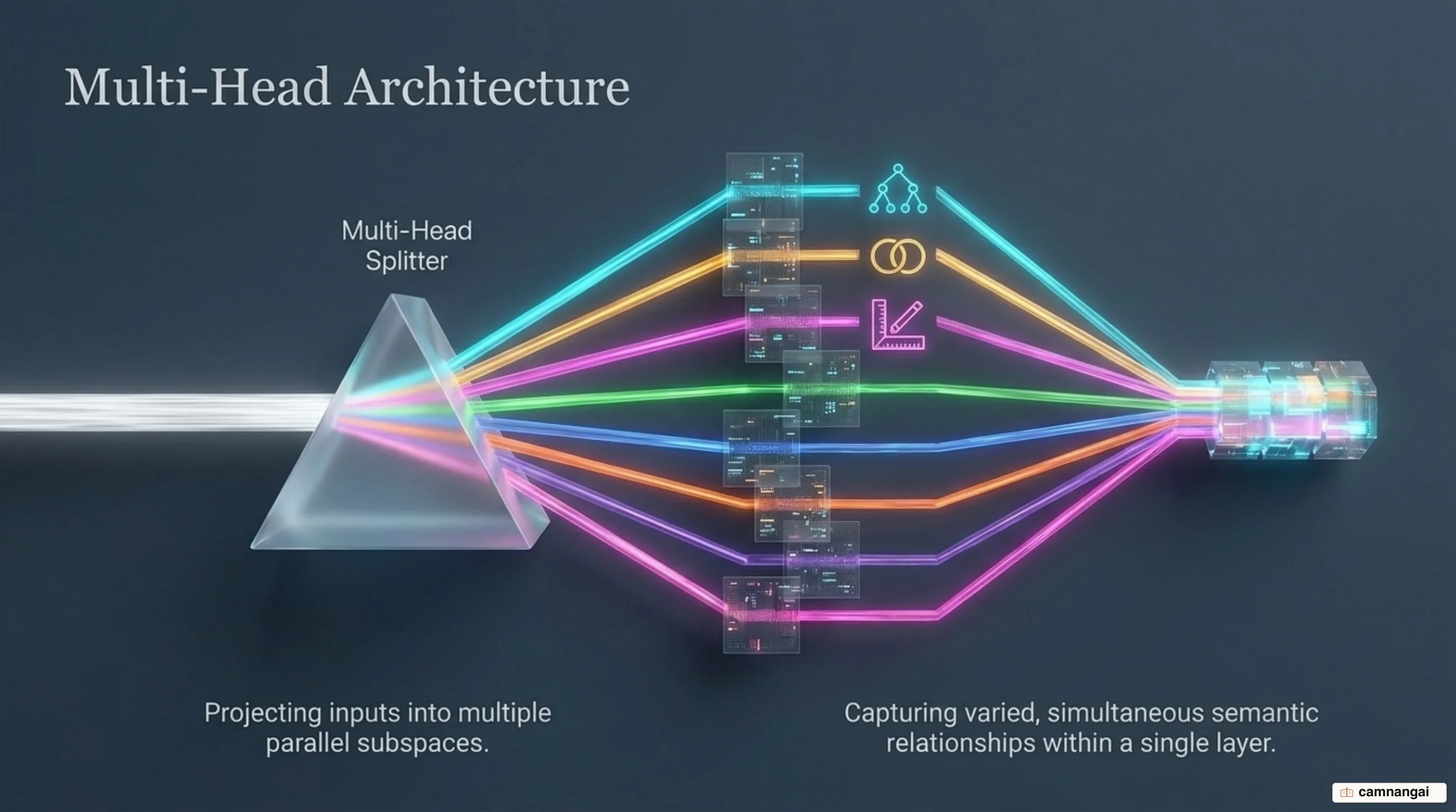
Single-head scaled dot-product attention suffers from a representational limitation: averaging attention distributions across an entire sequence under a single set of query-key projections forces the layer to compromise between competing linguistic dependencies. For example, a single attention head cannot simultaneously focus on immediate grammatical syntax (verb-object agreement) and distant semantic co-reference (subject-pronoun relationships) within the same token step.

Multi-Head Attention (MHA) resolves this constraint by projecting your queries, keys, and values h times using independent, learned linear transformations. This projects your input sequence into h distinct representation subspaces, executing scaled dot-product attention concurrently across all h heads:

text

MultiHead(Q, K, V) = Concat(head_1, head_2, ..., head_h) · W^O
head_i = Attention(Q · W_i^Q, K · W_i^K, V · W_i^V)

The dimensional projection parameters are defined as:

W_i^Q: projection matrix of dimension [d_model, d_k]
W_i^K: projection matrix of dimension [d_model, d_k]
W_i^V: projection matrix of dimension [d_model, d_v]
W^O: final projection matrix of dimension [h · d_v, d_model]

In standard Transformer setups (Vaswani et al., 2017), you configure hyperparameters to h = 8 parallel heads, model dimension d_model = 512, and per-head projection dimensions d_k = d_v = d_model / h = 64. To execute this efficiently on accelerator hardware, you do not instantiate h separate physical linear layers. Instead, you project your input tensor of shape (batch_size, sequence_length, 512) using a single unified linear matrix of size (512, 512) for queries, keys, and values. You then reshape and transpose the output tensor into (batch_size, 8, sequence_length, 64). Because the feature dimension per head is reduced to d_k = 64, the total computational complexity and parameter count of running h = 8 parallel heads match single-head attention executed at full model dimension (8 x 64 = 512). MHA expands your model's representation capacity without inflating FLOP overhead.

The O(N²) Computational Bottleneck and the Rise of FlashAttention

Despite the theoretical path-length advantages of self-attention, standard scaled dot-product attention encounters a computational wall when scaling to long contexts. Its runtime execution time and activation memory footprint scale quadratically O(N² · d) with sequence length N for hidden dimension d. Evaluating Q · K^T requires constructing and storing an intermediate N x N matrix of attention scores for every head across every transformer layer. When your sequence length N expands from 2,048 tokens to 32,768 or 100,000 tokens, the memory required to store uncompressed N x N attention activation maps rapidly exhausts accelerator VRAM capacity.

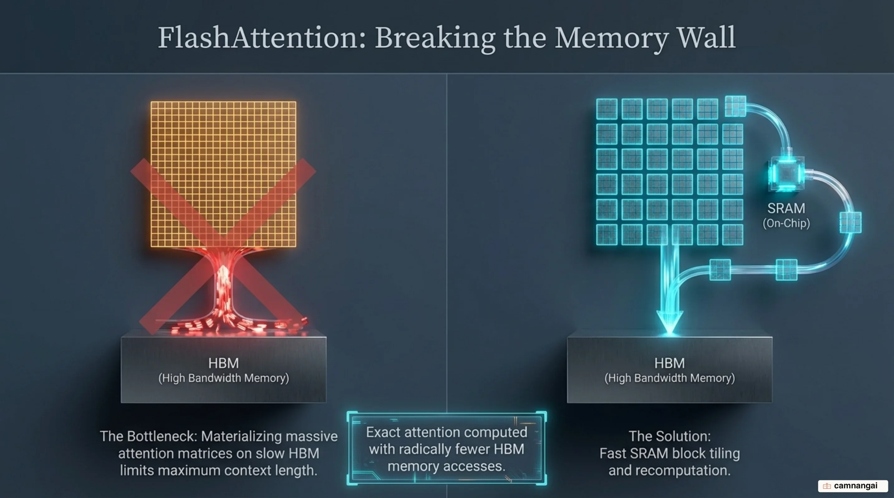
When you benchmark standard attention implementations on modern GPUs (such as NVIDIA A100s), performance stalls not from compute throughput constraints (FLOPs), but from hardware memory bandwidth bottlenecks (I/O limits). Modern GPUs feature two primary memory layers: a high-capacity, high-latency High-Bandwidth Memory (HBM, ~1.5–2.0 TB/s bandwidth, ~40–80 GB capacity) and a low-capacity, low-latency SRAM cache (~19 TB/s bandwidth, ~192 KB per Streaming Multiprocessor). In standard PyTorch implementations, your system reads Q and K from HBM into SRAM, computes S = (Q · K^T) / √d_k, writes the large N x N matrix S back out to HBM, reads S back into SRAM to evaluate softmax P = softmax(S), writes P back out to HBM, and finally reads P and V back into SRAM to compute output O = P · V. These repeated round-trip reads and writes of massive N x N matrices across high-latency memory buses stall GPU Tensor Cores, leaving them execution-bound by memory access delays.

FlashAttention (Dao et al., 2022) eliminates this hardware bottleneck by introducing an I/O-aware, exact attention algorithm that computes attention without materializing intermediate N x N matrices in HBM. FlashAttention structures attention algorithms to fit GPU memory hierarchies directly, loading sub-blocks of Query, Key, and Value matrices into fast SRAM, computing attention locally, and updating output tensors incrementally.

text

+--------------------------------------------------------------------+
|                   STANDARD ATTENTION (I/O BOUND)                   |
|                                                                    |
|  HBM (High-Bandwidth Memory)  <--->  GPU SRAM Cache (Registers)     |
|                                                                    |
|  Read Q, K  --------> Compute Q K^T --------> Write S [N x N]      |
|  Read S     --------> Compute Softmax ------> Write P [N x N]      |
|  Read P, V  --------> Compute P V ----------> Write Output O       |
|                                                                    |
|  * Result: High HBM Read/Write Overhead, Memory Limited O(N^2)     *|
+--------------------------------------------------------------------+
|                   FLASHATTENTION (I/O AWARE)                       |
|                                                                    |
|  HBM Memory                   GPU Fast SRAM Cache                  |
|                                                                    |
|  Stream Q_i, K_j, V_j Blocks  ---> Compute Tiled Local Softmax     |
|                               ---> Update Running Scaling Factors  |
|                               ---> Compute Tiled Local Output O_i  |
|                                                                    |
|  * Result: Zero N x N Matrices in HBM, Memory Limited O(N)         *|
+--------------------------------------------------------------------+

FlashAttention achieves exact mathematical identity with standard attention using two algorithmic strategies: Tiling and Recomputation.

Tiling: FlashAttention partitions inputs Q, K, V into blocks that fit into SRAM. In the forward pass, it streams key-value blocks through SRAM while updating local softmax normalization statistics online. By maintaining running scaling statistics, it computes exact output vectors block-by-block without storing intermediate N x N attention maps in HBM.
Recomputation: Instead of storing intermediate N x N attention probability matrices during the forward pass to use during backpropagation, FlashAttention stores only the target output vectors and online normalization parameters in HBM. During the backward pass, it recomputes attention scores block-by-block directly inside fast SRAM registers.

By reducing HBM memory access complexity from O(N²) to O(N) memory reads and writes, FlashAttention delivers a 2x to 4x wall-clock speedup during training while reducing memory footprints by over an order of magnitude. This optimization allows you to scale context windows dramatically without relying on lossy mathematical approximations.

Verdict: How Attention Reshaped Modern Model Architecture

Attention mechanisms redesigned modern deep learning system architecture by replacing rigid sequential recurrence and spatial convolution with dynamic, content-addressable routing. By reducing maximum sequence path lengths to O(1), attention layers eliminated historic gradient propagation constraints on long inputs and enabled complete intra-example parallelization during hardware training.

When you engineer modern sequence architectures, scaled dot-product multi-head attention is your core architectural primitive for modeling context interactions. When deploying models on standard context lengths (N <= 2048), standard GPU BLAS matrix operations execute with high efficiency. However, when you scale context windows where sequence length dominates model dimension, you should transition your pipeline to I/O-aware algorithms like FlashAttention. By combining block tiling and SRAM recomputation, I/O-aware attention removes hardware memory bandwidth constraints, enabling exact attention computation across long context sequences.