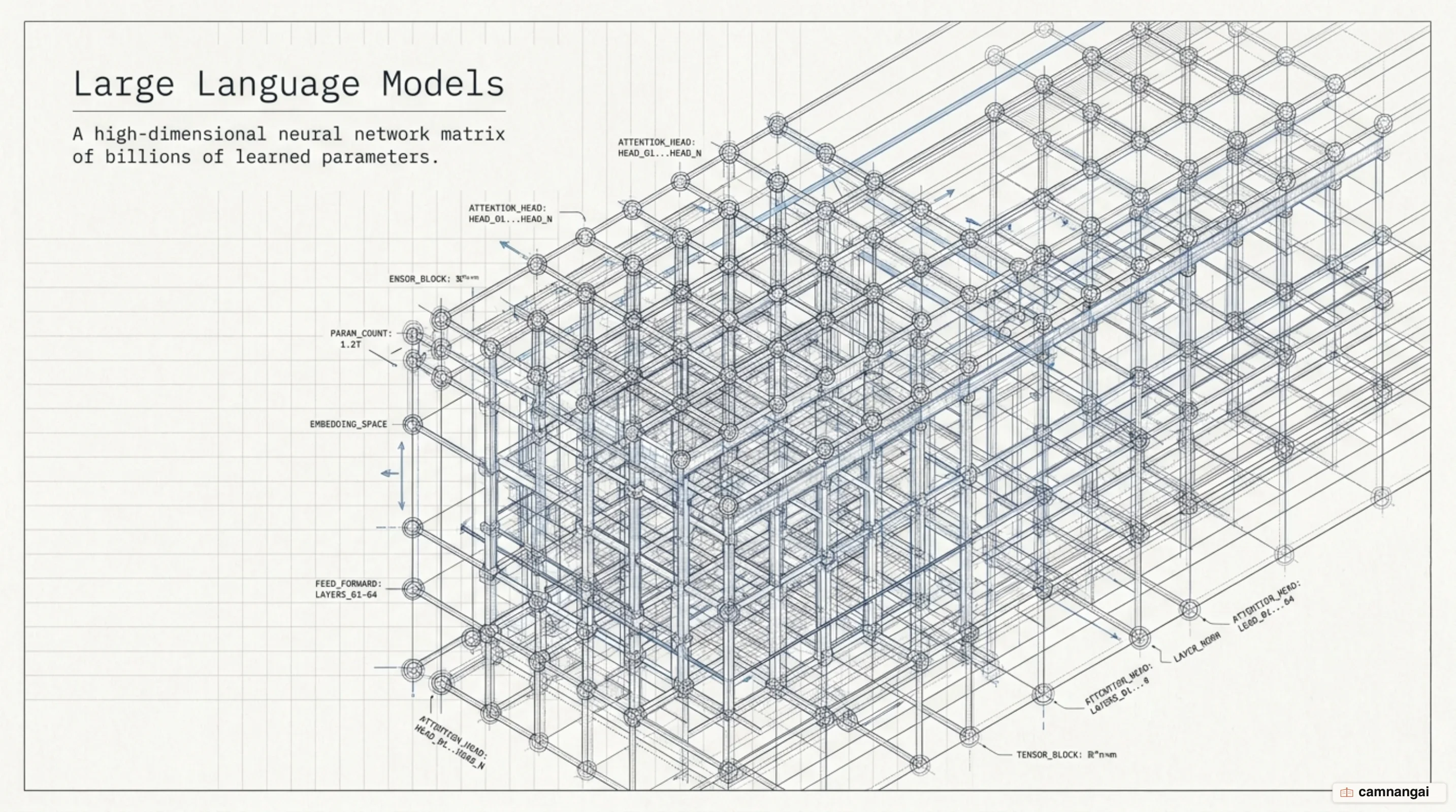
When you build, fine-tune, or deploy large language models, LLM parameters represent the internal learned weights and biases established during pretraining that determine how input signals are mathematically transformed into output token probabilities.
These numerical values form the structural memory and functional execution logic of the neural network, directly encoding linguistic structure, contextual relationships, and reasoning patterns into the model's weight matrices.
You must explicitly distinguish these learned internal parameters from external runtime inference hyperparameter knobs, such as temperature, top-p, or max output tokens. External inference parameters alter runtime probability sampling strategies and context truncation boundaries without modifying the underlying neural weights. In contrast, LLM parameters remain static during inference, forming the fixed high-dimensional matrix architecture through which runtime sampling mechanisms operate.
What are LLM parameters?
At a foundational level, parameters are trainable numerical values within a neural network that dictate
signal transformation across connected layers. In a single artificial neuron, an input vector X = (x_1, x_2, ..., x_n) undergoes a linear transformation calculated as:
z = w_1*x_1 + w_2*x_2 + ... + w_n*x_n + b
a = σ(z)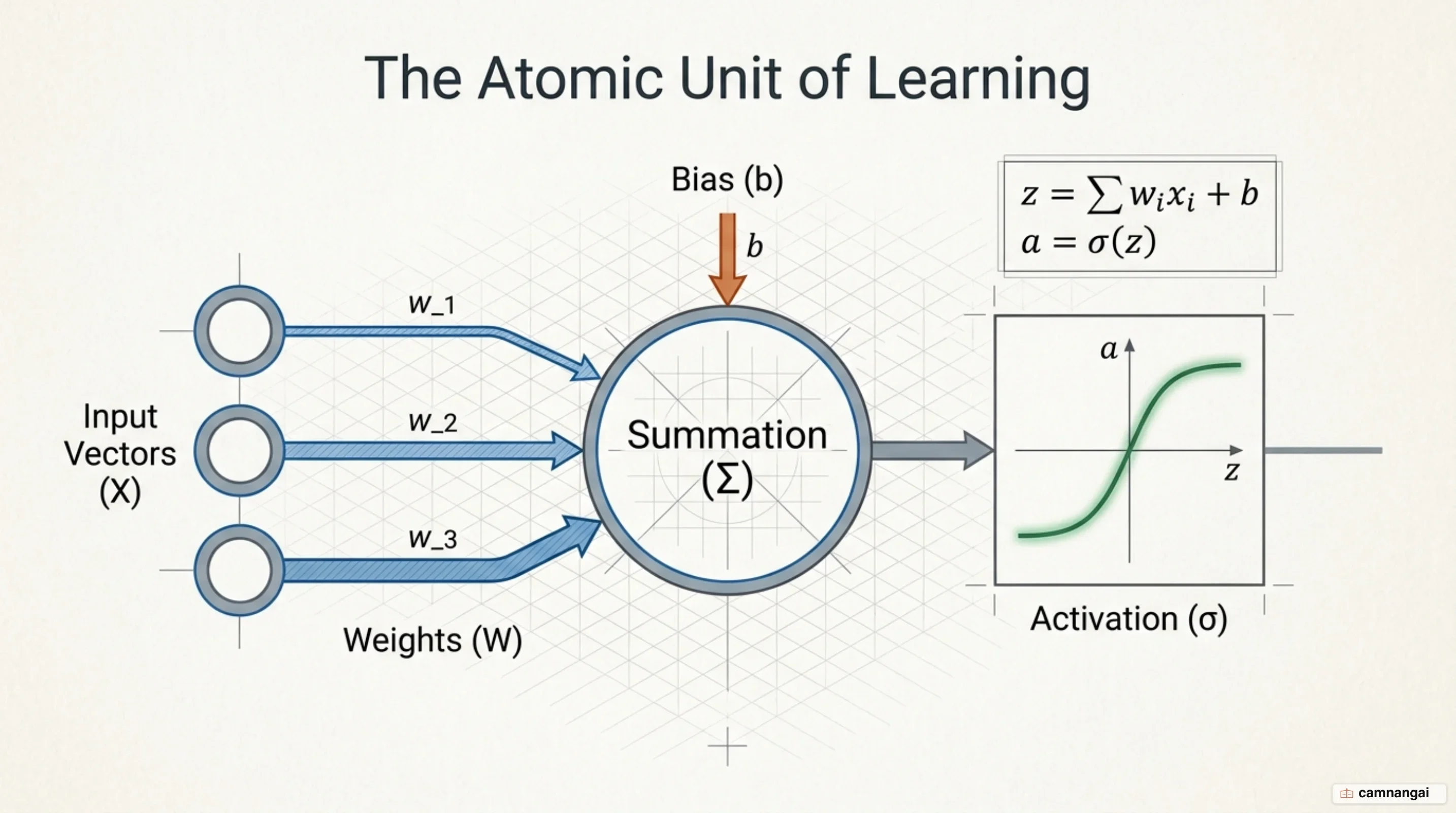
This scalar value z is subsequently passed through a non-linear activation function a = σ(z),
such as a Rectified Linear Unit (ReLU), Gaussian Error Linear Unit (GELU), or SwiGLU. The integration of
non-linear activations is mathematically essential to prevent linear collapse across deep architectures.
Without non-linearities, stacking multiple linear layers mathematically reduces to a single linear matrix
multiplication regardless of network depth, stripping the model of its ability to learn complex function
approximations.
Within this mathematical framework, weights (w_i) function as multiplicative scaling factors that
amplify or attenuate signal intensity, controlling the relative contribution of each input feature to
downstream activations. Biases (b) act as trainable offset vectors that shift the activation
threshold along the output axis independent of input signal magnitudes, ensuring neurons can fire even
when input vectors are zero or weakly expressed.
Transformer-based large language models scale these basic transformations across billions of parameters structured within stacked multi-head self-attention mechanisms and dense feed-forward network (FFN) blocks. By executing sequential high-dimensional matrix multiplications, the parameter architecture processes input token embeddings into contextualized internal representations, ultimately mapping sequence history to a probability distribution over the vocabulary space.
How parameters learn during training
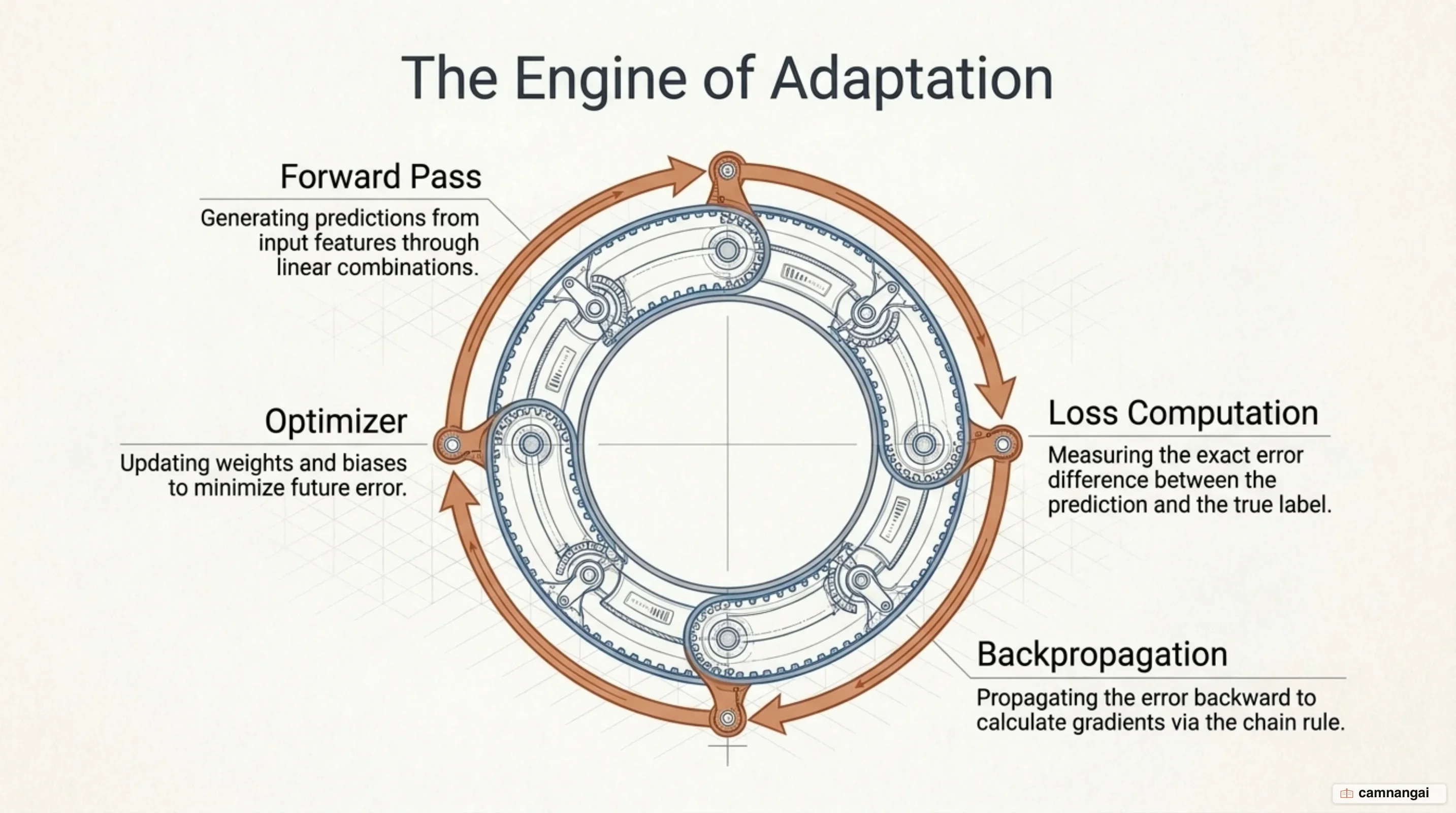
LLM parameters acquire their functional weights during an iterative pretraining phase on large-scale textual corpora. This optimization process operates through a structured four-step lifecycle:
- Forward Pass: Input token sequences are converted into high-dimensional embeddings and passed through the network's attention and feed-forward layers. Linear tensor operations and non-linear activations produce a final logit matrix, which a softmax function transforms into predicted output token probabilities.
- Error Calculation: An objective loss function (typically cross-entropy) measures the divergence between the model's predicted probability distribution and the ground-truth target tokens, yielding a scalar loss value.
- Backward Pass (Backpropagation): The scalar error is propagated backward through every layer using the partial derivative chain rule of calculus. On a hardware level, this step requires allocating dedicated gradient memory buffers matching the exact shapes of the model's parameter tensors. GPUs execute matrix transpose operations and compute partial derivatives for every weight matrix to quantify its exact contribution to the total loss.
- Weight Update: An optimization algorithm—such as Adam or Stochastic Gradient Descent (SGD)—adjusts parameter values in the opposite direction of the calculated gradients. When using Adam, the optimizer maintains auxiliary parameter states (first and second momentum vectors) to dynamically scale updates based on historical gradient variance, iteratively minimizing global loss.
Parameter states are dynamic during training, constantly modified by optimizer states, gradient allocations, and backpropagation steps. During inference, these parameter matrices are frozen, operating as static execution kernels that transform inputs without altering internal values.
If parameter capacity is excessively large relative to the volume, diversity, and quality of the training dataset, the model risks overfitting. In an overfitted state, parameter weight matrices memorize specific training sequences rather than learning generalized language representations, leading to degraded performance on unseen evaluation data.
Chinchilla scaling laws: are bigger models always better?
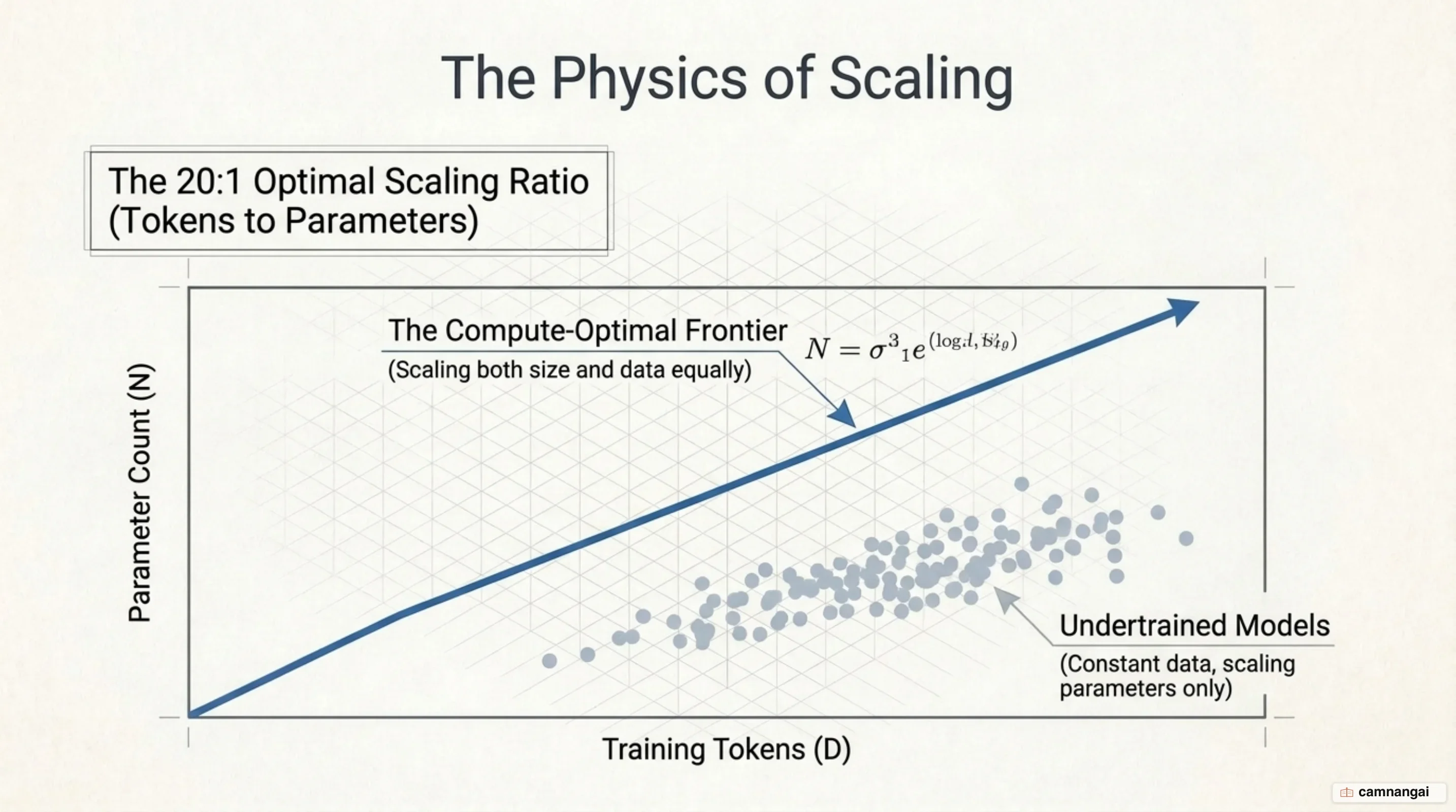
Historically, model development prioritized parameter scaling over training dataset expansion. Frontier architectures such as GPT-3 (175 billion parameters) and Gopher (280 billion parameters) scaled weight capacity aggressively while keeping training token volumes static at roughly 300 billion tokens. Empirical research by Hoffmann et al. (2022) revealed that this paradigm left models severely undertrained relative to their total compute budgets, wasting compute allocations on excess parameter capacity that lacked sufficient data exposure to converge.
Hoffmann et al. established the Chinchilla compute-optimal scaling laws, proving that for a fixed compute budget, model parameter count and training dataset volume must be scaled in equal 1:1 proportions. Compute-optimal convergence dictates a constant ratio of approximately 20 tokens per parameter.
This theoretical scaling law was validated by comparing DeepMind's Gopher (280B parameters trained on 300B tokens) against Chinchilla (70B parameters trained on 1.4 trillion tokens). Trained under the exact same total FLOP compute budget, Chinchilla used a model one-fourth the size of Gopher paired with nearly five times more training data.
Chinchilla uniformly outperformed larger, undertrained models across downstream benchmarks, achieving an average accuracy of 67.5% on the MMLU evaluation—a 7% improvement over Gopher. Beyond benchmark accuracy, compute-optimal sizing provides direct operational advantages: deploying a 70B parameter model instead of a 280B model drastically reduces GPU VRAM allocation, lowers hardware infrastructure footprints, and significantly reduces generation latency during fine-tuning and production inference.
MoE architecture: total vs. active parameters
Sparse Mixture of Experts (MoE) architectures decouple total parameter footprint from per-token compute FLOPs. In a standard dense transformer model, 100% of the parameter weights participate in every forward pass calculation for every input token. In contrast, sparse MoE architectures replace dense feed-forward network (FFN) layers with sparse MoE layers containing multiple parallel expert sub-networks regulated by a learned gating router.
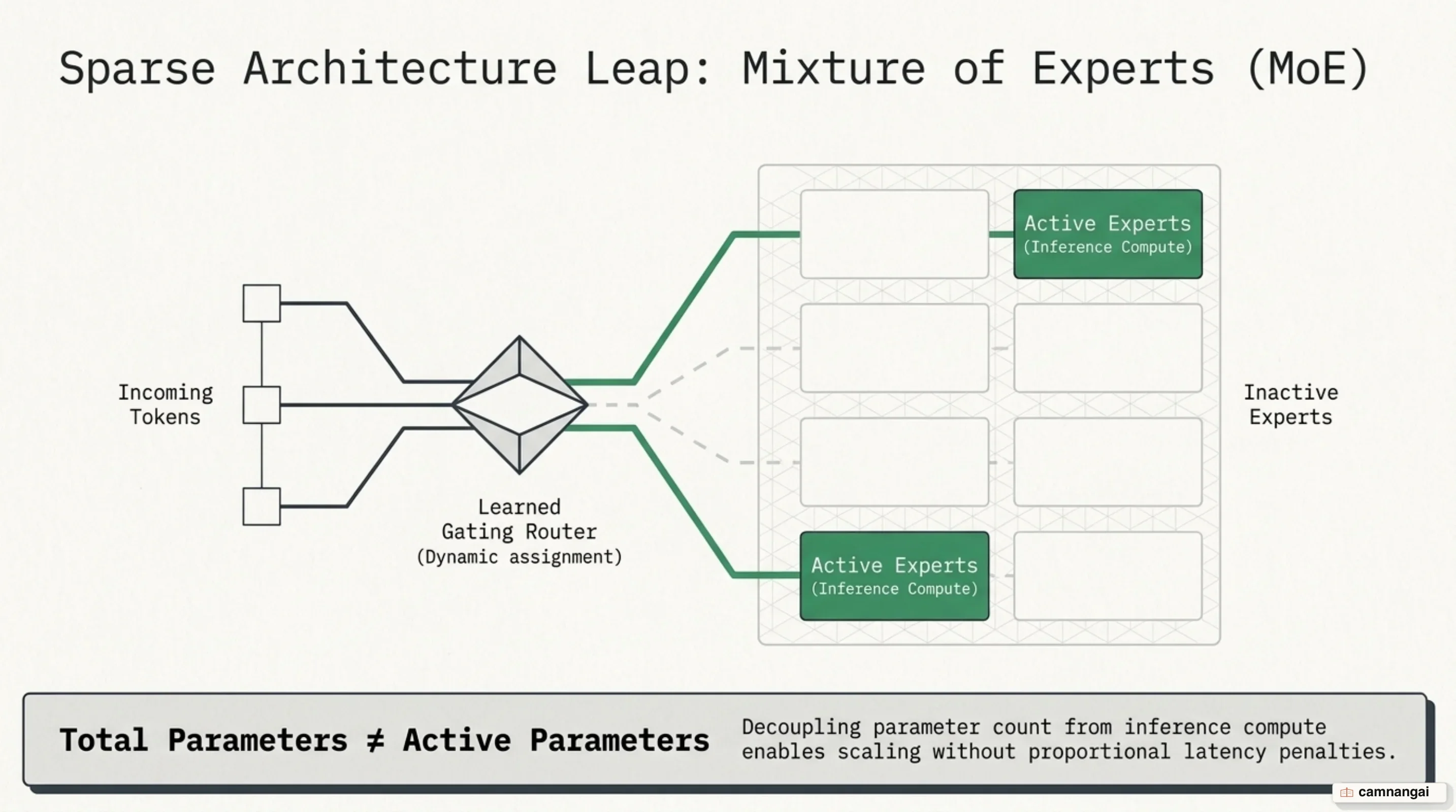
The gating router evaluates incoming token representations and dynamically assigns them to specific experts (typically utilizing top-1 or top-2 selection rules). To ensure computational efficiency across hardware clusters, MoE training enforces expert capacity limits and incorporates auxiliary load-balancing losses, preventing token routing bottlenecks and ensuring uniform workload distribution across expert sub-networks.
Mixtral 8x7B provides a concrete example of sparse MoE parameter dynamics:
- Total Parameter Calculation: While composed of eight nominal 7-billion parameter expert blocks, Mixtral 8x7B contains approximately 47 billion total parameters rather than 56 billion (8 × 7B). This occurs because critical non-FFN architecture components—such as multi-head self-attention projections, layer normalization, and token embeddings—are shared globally across all experts.
- Active Parameter Footprint: Operating with top-2 expert routing per token, Mixtral routes inputs through two active experts per MoE layer alongside the shared attention blocks. This results in an active compute footprint using ~12B to 14B parameters worth of FLOP calculations per token forward pass, rather than evaluating the entire 47B matrix footprint.
- VRAM Memory Overhead: Despite executing FLOP calculations equivalent to a ~12B dense model, all 47 billion total parameters must remain fully loaded in GPU VRAM. Because any incoming token can dynamically trigger any expert sub-network at runtime, the complete parameter footprint must reside in system memory.
Calculating VRAM and hardware requirements in practice
Determining GPU VRAM allocation for deployment requires calculating baseline static parameter memory alongside dynamic runtime execution buffers. Base memory consumption per parameter is strictly dictated by numeric precision (data type):
- FP32 (Full Precision): 4 bytes per parameter
- FP16 / BF16 (Half Precision): 2 bytes per parameter
- INT8 (8-bit Quantization): 1 byte per parameter
- INT4 (4-bit Quantization): 0.5 bytes per parameter
To estimate the static VRAM required to load model weights into GPU memory, use the formula:
Memory (Bytes) = Parameter Count × Bytes per ParameterDeploying models in production environments requires factoring in additional dynamic overhead:
- Inference Overhead: You must allocate a baseline ~20% memory buffer above static parameter weights to accommodate key-value (KV) cache expansion, activation buffers, and framework context structures. However, for long-context generation or high concurrency batch sizes, the KV cache footprint scales linearly with sequence length and batch size, which will rapidly exceed the default 20% baseline allocation.
- Training Overhead: Standard model training using the Adam optimizer requires approximately 4x the base parameter memory footprint in VRAM. This capacity stores optimizer states (first and second momentum vectors), weight gradients, and intermediate activation checkpoints required for backpropagation.
The table below outlines static loading memory and recommended production inference memory (inclusive of the baseline +20% runtime buffer) across key parameter tiers and precision dtypes:
| Model Tier | Precision Dtype | Bytes / Param | Static Loading Memory | Recommended Inference Memory (+20%) |
|---|---|---|---|---|
| 8B Parameters | FP16 / BF16 | 2.0 B | 16.0 GB | 19.2 GB |
| INT8 | 1.0 B | 8.0 GB | 9.6 GB | |
| INT4 | 0.5 B | 4.0 GB | 4.8 GB | |
| Mixtral 8x7B (47B) | FP16 / BF16 | 2.0 B | 94.0 GB | 112.8 GB |
| INT8 | 1.0 B | 47.0 GB | 56.4 GB | |
| INT4 | 0.5 B | 23.5 GB | 28.2 GB | |
| 70B Parameters | FP16 / BF16 | 2.0 B | 140.0 GB | 168.0 GB |
| INT8 | 1.0 B | 70.0 GB | 84.0 GB | |
| INT4 | 0.5 B | 35.0 GB | 42.0 GB |
Key takeaways
- Parameter Definition: Internal learned weights and biases that define model behavior, fundamentally separate from static external runtime parameters.
- Mathematical Execution: Neuronal transformations rely on linear weight-signal scaling and bias shifting followed by non-linear activations.
- Compute-Optimal Scaling: Following Chinchilla laws, model sizing and training token volume must scale equally (~20 tokens per parameter).
- Sparse MoE Allocation: MoE architectures separate total memory footprint from active compute FLOPs; full parameter weights must stay loaded in VRAM regardless of active per-token routing.
- VRAM Calculation: Model footprint scales strictly by numeric precision (2 bytes for FP16, 0.5 bytes for INT4); inference requires a ~20% buffer for KV cache and activations, while Adam training requires ~4x base parameter size.