Model scaling drives modern , but it introduces severe infrastructure bottlenecks. When you train or serve large language models () containing tens or hundreds of billions of parameters, a single GPU reaches memory saturation almost immediately. Executing these deep architectures requires holding , active gradients, optimizer states, and intermediate activations or key-value (KV) caches. Distributed Training and distributed inference architectures eliminate this physical memory wall by partitioning compute workloads across multi-GPU and multi-node compute clusters.
During model execution, memory consumption splits between static state requirements and dynamic runtime tensors. Training demands substantial VRAM to store full-precision master weights, momentum, and variance vectors alongside intermediate forward-pass activations retained for backpropagation. Conversely, online inference eliminates gradient tracking and optimizer state allocation entirely, but introduces dynamic key-value (KV) cache allocations that scale proportionally with context sequence length and concurrent request volume.
Orchestrating operations across distributed environments requires precise coordination between execution paradigms, parallelization topologies, and underlying hardware interconnects. Selecting optimal configurations demands balancing compute-bound vector matrix operations against communication-bound collective operations across high-speed NVLink channels and inter-node network fabrics.
The Memory Wall: Why a Single GPU Is Never Enough
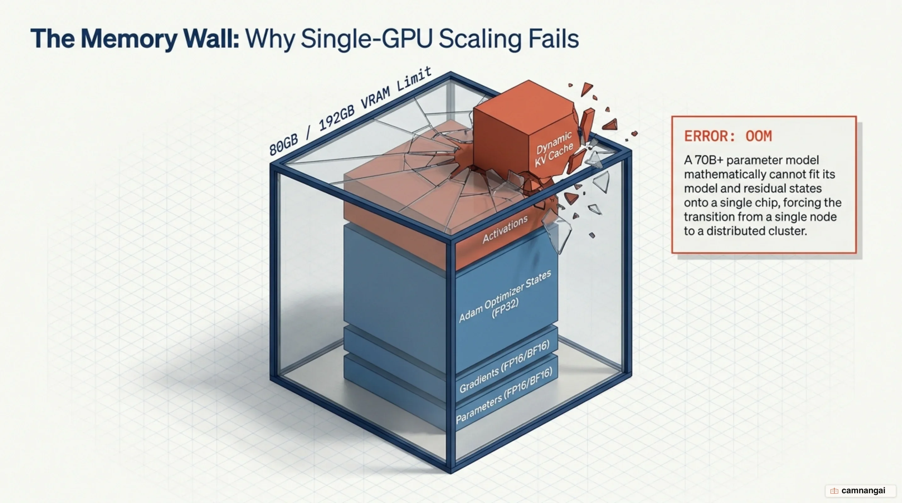
Executing large on a single accelerator is restricted by physical VRAM capacity. Memory during execution is consumed by four primary components: model parameters, model gradients, optimizer states, and intermediate activations. While static model parameters establish the baseline memory footprint, dynamic components generated during numerical optimization and forward-pass tracking scale memory demands beyond the hardware limits of individual devices.
The mathematical memory footprint of mixed-precision training demonstrates why single-GPU VRAM saturates rapidly. In 16-bit precision (FP16 or BF16), model parameters consume 2 bytes per parameter. However, maintaining numerical stability during optimization via algorithms like Adam requires maintaining a 32-bit (FP32) master copy of the weights at 4 bytes per parameter, an FP32 gradient tensor at 4 bytes per parameter, and Adam optimizer states (which track first-moment momentum and second-moment variance) at 8 bytes per parameter (4 bytes each). Consequently, static model states require 16 bytes of VRAM per parameter:
Memory_static = 2 bytes (FP16 params) + 4 bytes (FP32 params) + 4 bytes (FP32 grads) + 8 bytes (Adam states) = 16 bytes/param
A 10-billion parameter model therefore requires 160 GB of VRAM solely for static model states before allocating memory for intermediate feature maps, temporary execution buffers, or workspace memory fragmentation.
Training memory profiles contrast sharply with serving memory profiles. Inference eliminates the 12 bytes per parameter assigned to gradients and Adam optimizer states, leaving VRAM dominated by static model weights (2 bytes per parameter in FP16/BF16) and dynamic key-value (KV) caches. While training memory scales with batch size and sequence length via intermediate activation tensors stored for backpropagation, inference memory scales primarily with context length, concurrent request throughput, and allocated KV cache blocks during auto-regressive decoding.
To manage activation memory overhead during training, system architects rely on activation recomputation (gradient checkpointing). Instead of storing all intermediate feature maps across every layer during the forward pass, activation recomputation retains tensors only at designated partition boundaries. During the backward pass, non-retained intermediate activations are recomputed on-demand through an extra local forward pass. This reduces activation memory space complexity from linear $O(L)$ relative to layer depth $L$ down to O(sqrt(L)), trading extra forward pass compute operations for capacity. System designers can also deploy selective activation recomputation, which retains heavy attention tensors while recomputing lightweight point-wise operations like GELU and LayerNorm.
Parallelism Strategies: Data, Tensor, and Pipeline Parallelism
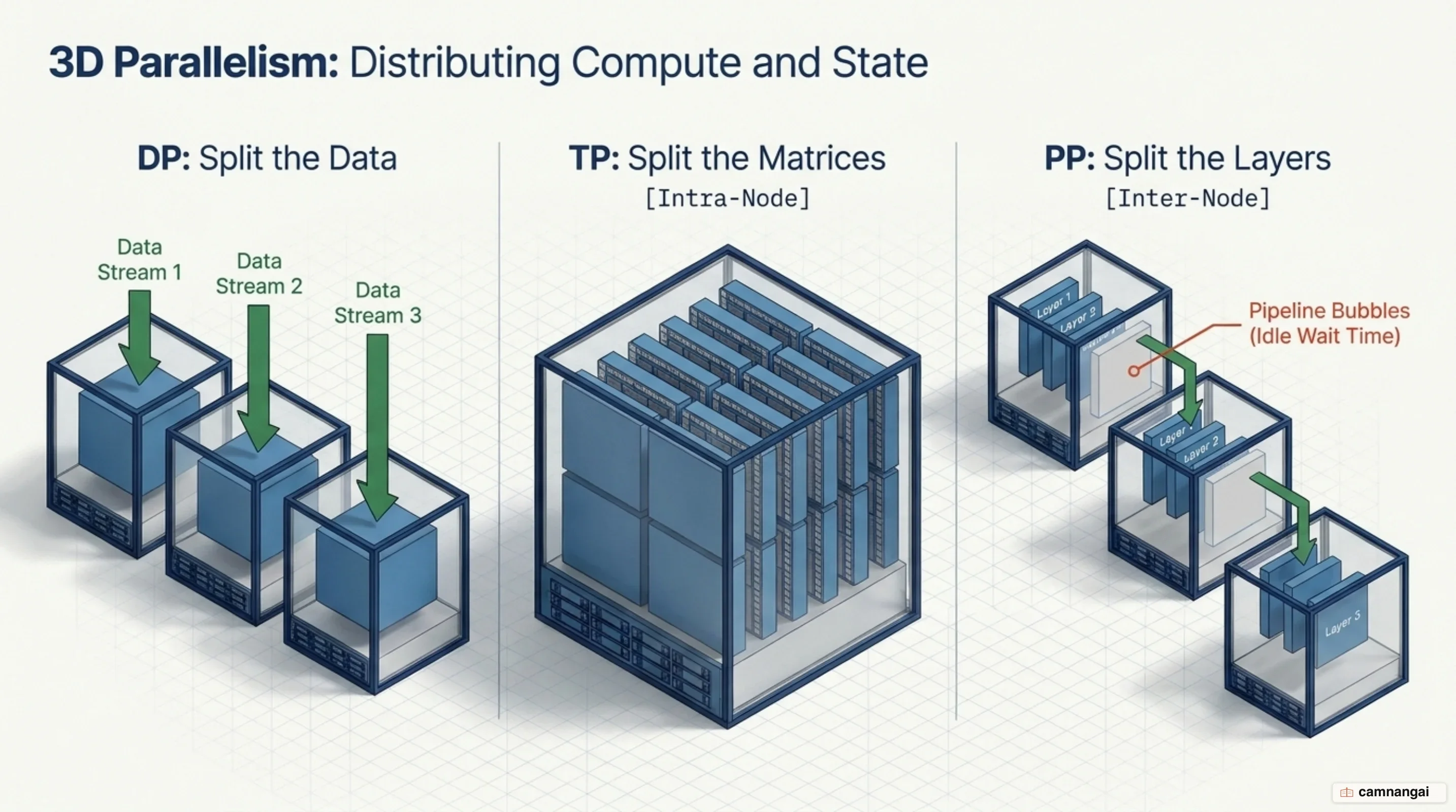
When a model or its runtime states exceed single-GPU capacity, you must split the workload across multiple accelerators using data, tensor, or pipeline parallelism. Distributed Data Parallelism (DDP) duplicates the complete model architecture across every worker GPU while splitting the training dataset across mini-batches. Each rank independently executes a forward and backward pass over its local data batch. Once gradients are calculated, ranks execute an AllReduce collective operation to synchronize gradients across the cluster before updating parameters. DDP optimizes throughput by bucketing individual parameter gradients into contiguous memory buffers, overlapping gradient communication asynchronously with the backward pass computation of preceding layers.
Tensor Parallelism (TP) horizontally partitions individual weight matrices across multiple GPUs within a single layer. In a Multi-Layer Perceptron (MLP) block, General Matrix Multiplications (GEMM) are split using column-parallel and row-parallel linear layers. The first linear layer splits the weight matrix along its columns, evaluating partitioned outputs in parallel across ranks. The second linear layer splits its weight matrix along rows, multiplying local activation shards before invoking an intra-layer AllReduce collective to aggregate the final hidden states. To further optimize memory, Tensor Parallelism is frequently combined with Sequence Parallelism (SP). Sequence Parallelism splits activation memory across the sequence dimension during LayerNorm and Dropout operations using AllGather and ReduceScatter primitives, eliminating activation memory bottlenecks inside TP worker groups.
import torch
import torch.nn as nn
import torch.distributed as dist

class TensorParallelMLP(nn.Module):
    def __init__(self, hidden_size: int, ffn_size: int, world_size: int):
        super().__init__()
        self.rank_ffn_size = ffn_size // world_size
        # Column-parallel linear layer (splits weight matrix along output dimension)
        self.w1 = nn.Parameter(torch.empty(self.rank_ffn_size, hidden_size))
        # Row-parallel linear layer (splits weight matrix along input dimension)
        self.w2 = nn.Parameter(torch.empty(hidden_size, self.rank_ffn_size))

    def forward(self, x: torch.Tensor) -> torch.Tensor:
        # Step 1: Column-parallel GEMM + GeLU activation
        hidden_parallel = torch.matmul(x, self.w1.t())
        hidden_parallel = torch.nn.functional.gelu(hidden_parallel)

        # Step 2: Row-parallel GEMM
        output_parallel = torch.matmul(hidden_parallel, self.w2.t())

        # Step 3: Synchronize full hidden states via intra-layer AllReduce
        dist.all_reduce(output_parallel, op=dist.ReduceOp.SUM)
        return output_parallel
Pipeline Parallelism (PP) splits a model vertically by grouping consecutive layers into stages assigned to separate physical GPUs. Because sequential layer dependencies cause idle GPU waiting periods ("pipeline bubbles"), pipeline execution splits mini-batches into smaller micro-batches. Synchronous GPipe schedules process micro-batches sequentially across stages before aggregating gradients globally, incurring a bubble overhead fraction equal to:
Bubble Fraction = (d - 1) / (m + d - 1)
where $d$ represents the pipeline depth (number of stages) and $m$ represents the number of micro-batches. To reduce memory consumed by stored micro-batch activations, PipeDream implements a One Forward, One Backward (1F1B) schedule. Each worker alternates between executing one forward micro-batch and one backward micro-batch, using weight stashing or double-buffered weights (2BW) to maintain parameter consistency across execution passes.
Memory Optimization with ZeRO and FSDP
The Zero Redundancy Optimizer (ZeRO) eliminates memory redundancies in data-parallel training by partitioning model states across data-parallel ranks rather than replicating them. ZeRO functions in three incremental stages:
- ZeRO-1: Partitions 32-bit Adam optimizer states across data-parallel ranks, reducing VRAM demands by up to 4x while keeping communication volume identical to standard DDP.
- ZeRO-2: Partitions gradients alongside optimizer states, ensuring each rank retains only the gradients corresponding to its assigned optimizer partition.
- ZeRO-3 / FSDP: Partitions model parameters, gradients, and optimizer states across all data-parallel ranks. Parameters are represented as sharded tensors (such as PyTorch DTensor with
Shard(dim=0)). During execution, AllGather collectives dynamically reconstruct full parameters immediately before forward and backward passes, while ReduceScatter collectives shard computed gradients back across ranks.
To scale model training to trillion-parameter architectures, ZeRO-Infinity extends ZeRO-3 with an offload engine that moves parameters, gradients, and optimizer states to host CPU memory or NVMe storage. By incorporating memory-centric tiling (TiledLinear), ZeRO-Infinity breaks large linear operators into smaller sequential tiles executed in a loop. This design caps peak working memory requirements on the GPU without overwhelming host memory bandwidth.
PyTorch Fully Sharded Data Parallel 2 (FSDP2) introduces structural improvements over FSDP1 by adopting explicit DTensors sharded along dimension 0 (Shard(dim=0)). FSDP2 replaces flat-parameter abstractions with per-parameter tracking, enabling communication-free state dict management, meta-device initialization, and direct integration with torch.compile. It replaces CUDA stream management mechanisms (recordStream) with deterministic memory allocations that eliminate CPU synchronization stalls. FSDP2 offers explicit prefetching (set_modules_to_forward_prefetch), customizable mixed-precision policies, and custom tensor subclass extension points (such as native support for Float8 linears and NF4 for QLoRA). Ranks can inspect local parameter shards using param.to_local().
import torch
import torch.nn as nn
from torch.distributed.fsdp import fully_shard, MixedPrecisionPolicy

# Define mixed precision policy: BF16 compute, FP32 gradient reduction
mp_policy = MixedPrecisionPolicy(
    param_dtype=torch.bfloat16,
    reduce_dtype=torch.float32,
)

# Initialize model under FSDP2
model = MyTransformerBlock()

# Apply fully_shard to submodules first, then root model
for layer in model.layers:
    fully_shard(layer, mp_policy=mp_policy)
fully_shard(model, mp_policy=mp_policy)

# Initialize optimizer over sharded DTensor parameters
optimizer = torch.optim.Adam(model.parameters(), lr=1e-4)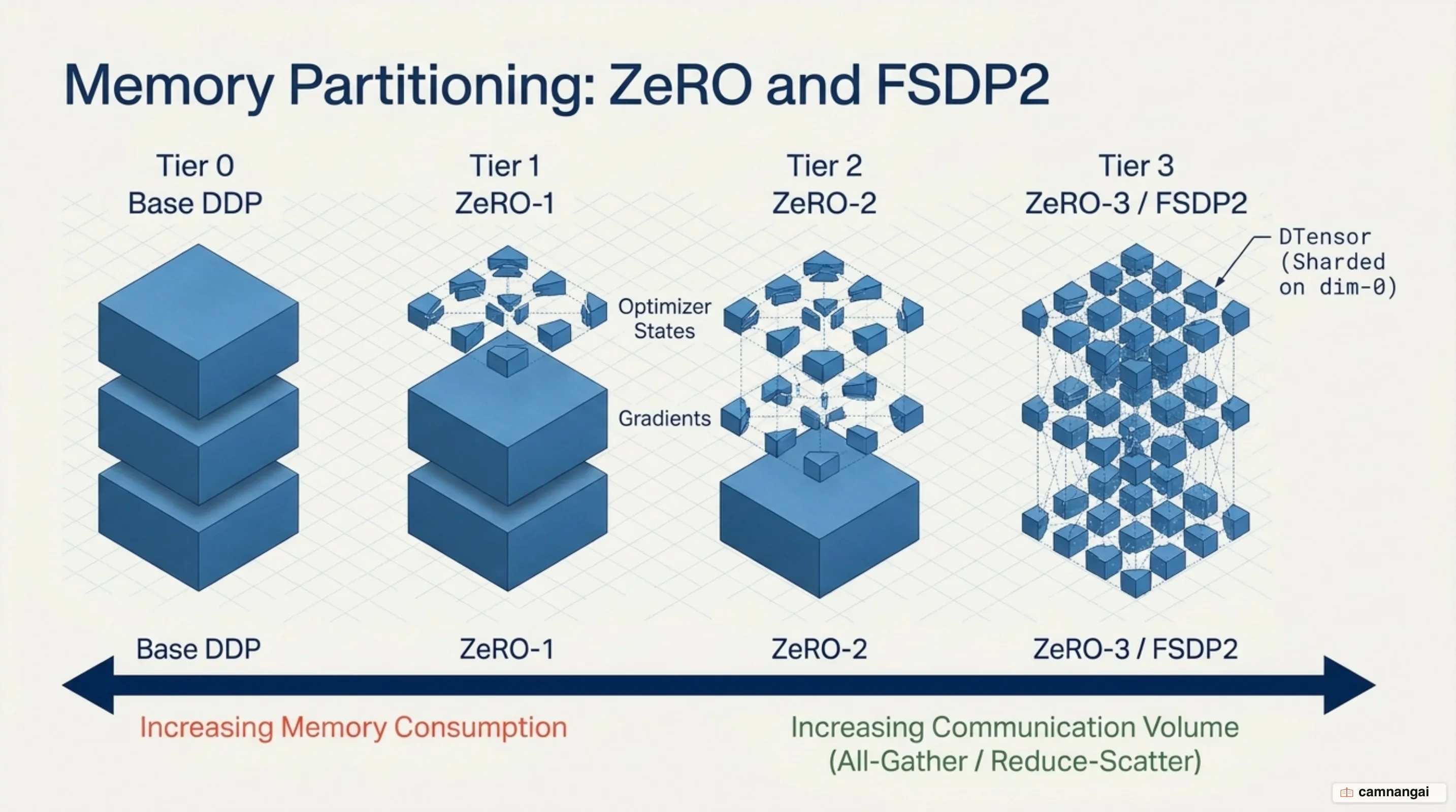
Distributed Inference: Latency Reduction and Serving Throughput
Distributed inference operates under different optimization goals than distributed training. Training maximizes aggregate throughput across large mini-batches over long execution horizons. Online serving must maximize throughput while satisfying strict Service Level Objectives (SLOs) bound to user-facing latency metrics. Serving performance is evaluated using two primary Key Performance Indicators (KPIs):
- Time to First Token (TTFT): The prefill phase latency required to process prompt input tokens and generate the initial output token.
- Time per Output Token (TPOT): The decode phase latency for generating each subsequent token auto-regressively.
Selecting an optimal distributed serving deployment depends on model scale, batching constraints, and cluster topology:
- Single GPU: Used when model parameters and active KV cache fit within a single accelerator's VRAM.
- Single-Node Multi-GPU: Employs Tensor Parallelism (TP) across GPUs to split intra-layer matrix operations over high-speed NVLink backplanes.
- Multi-Node Multi-GPU: Combines intra-node Tensor Parallelism with inter-node Pipeline Parallelism (PP). Intra-node TP accelerates high-frequency matrix operations, while inter-node PP splits layers across host nodes without introducing cross-node GEMM split latency.
During engine startup, serving frameworks like vLLM report available memory in terms of allocated GPU memory blocks. You can calculate the maximum concurrent token capacity of a node configuration by taking the logged # GPU blocks value and multiplying it by the block size (16 tokens). Serving engines manage runtime process execution using Python multiprocessing (mp) or Ray cluster management (ray). Single-node serving defaults to multiprocessing (mp) to minimize execution overhead, whereas multi-node serving requires Ray (ray) to coordinate worker processes, manage containerized environments, and synchronize execution placement across host nodes.
# Serve a large language model across 2 nodes using 8 GPUs per node (TP=8, PP=2)
vllm serve /path/to/model/weights \
    --tensor-parallel-size 8 \
    --pipeline-parallel-size 2 \
    --distributed-executor-backend ray
Disaggregated Prefill and Decode Architecture
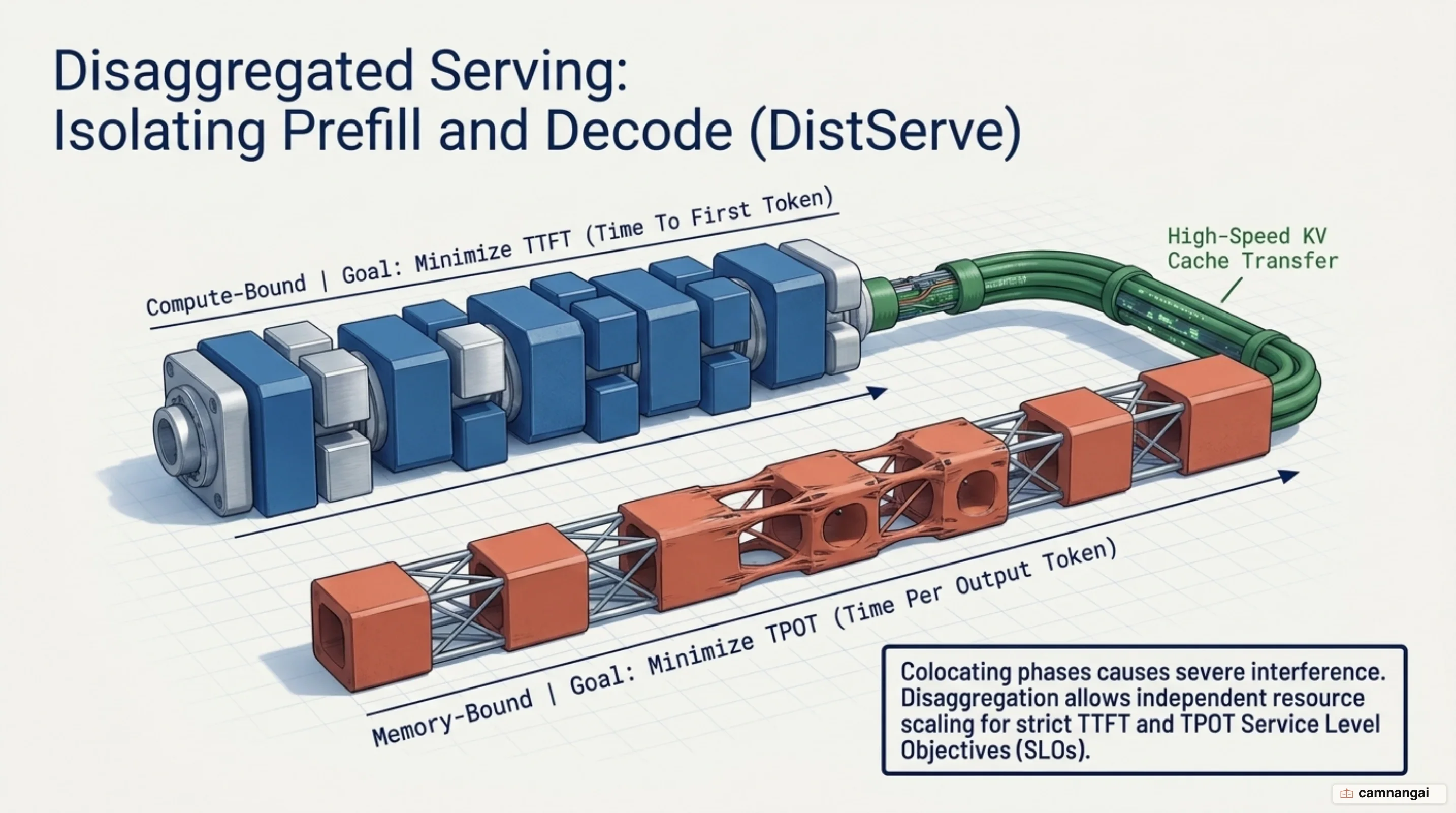
Monolithic serving engines execute prompt prefill and token decoding phases on the same set of co-located GPUs. However, these two execution phases exhibit conflicting computational profiles:
- Prefill Phase: Highly compute-bound. It processes long prompt token sequences simultaneously, fully saturating GPU Tensor Cores through large matrix-matrix multiplications.
- Decode Phase: Highly memory-bandwidth bound. It processes one token at a time per request, requiring repeated reads of model weight matrices and KV caches from VRAM for small vector-matrix operations.
In co-located serving systems, batching compute-bound prefill tasks alongside memory-bound decode requests introduces severe prefill-decoding interference. Compute-heavy prefill bursts monopolize GPU execution units, causing iteration time spikes that disrupt concurrent decode steps. This interference creates severe TPOT latency tail spikes. To maintain SLO compliance during load surges, operators are often forced to over-provision GPU infrastructure, reducing overall cluster efficiency.
DistServe resolves this bottleneck by disaggregating prefill and decode operations onto dedicated, physically isolated GPU clusters. By separating compute resources, prefill-decoding interference is eliminated. Disaggregation allows system engineers to customize parallelism plans for each phase independently—optimizing prefill nodes for TTFT latency targets and decode nodes for TPOT latency targets.
When a prefill node finishes processing an input prompt, it transfers the generated key-value (KV) cache tensors across the network interconnect to a decode node. DistServe co-optimizes resource allocation and network placement based on cluster interconnect bandwidth to minimize KV cache transfer overhead. By eliminating resource contention and tailoring execution plans per phase, disaggregated serving can achieve up to 7.4x higher request throughput or adhere to 12.6x tighter latency SLOs compared to co-located engines.
Interconnect Infrastructure: NVLink, InfiniBand, and NCCL
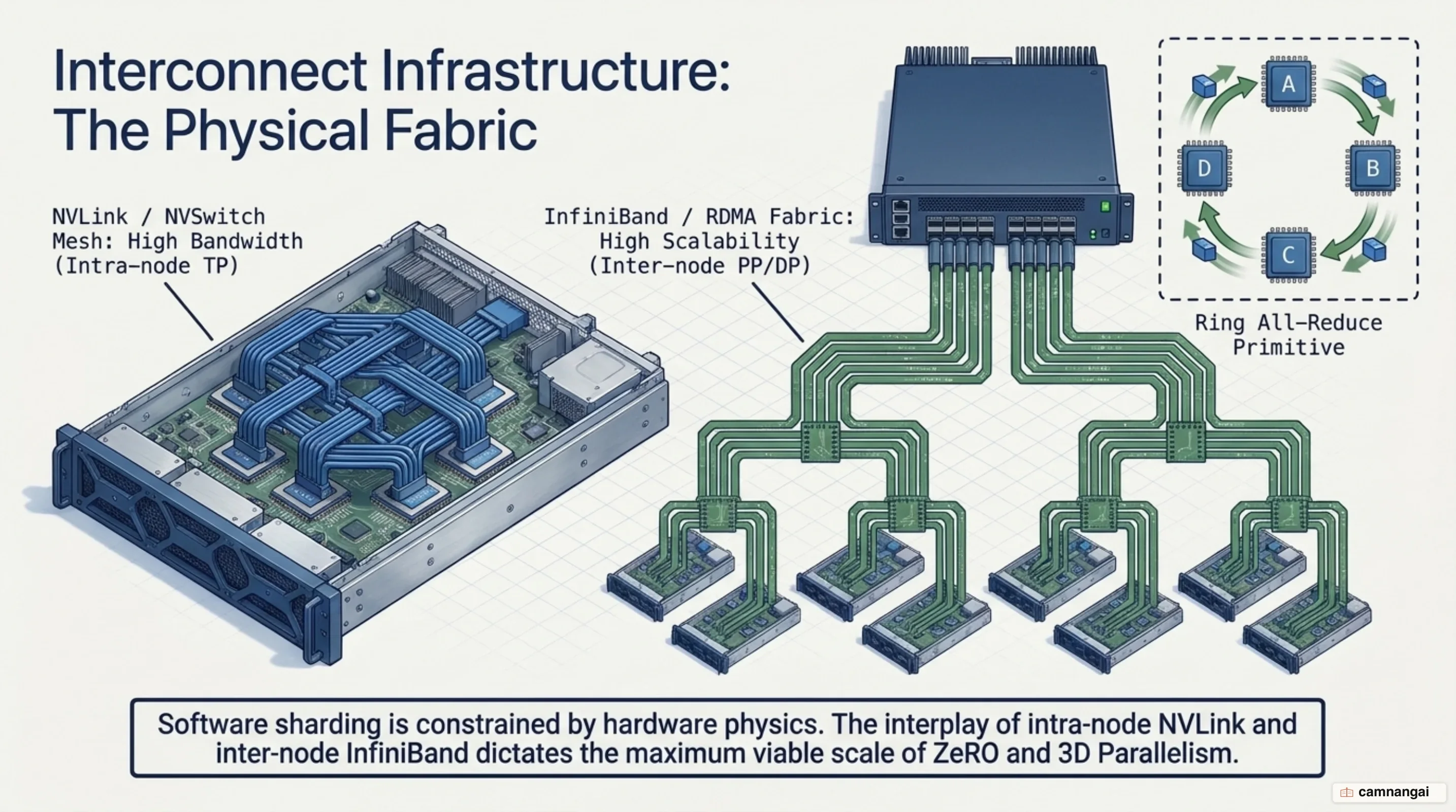
Distributed execution relies on the underlying cluster network topology. Hardware interconnects are structured hierarchically into intra-node and inter-node layers:
- Intra-Node Interconnects: Technologies like NVIDIA NVLink and NVSwitch provide high-bandwidth, direct GPU-to-GPU communications (reaching hundreds of gigabytes per second bidirectionally per GPU).
- Inter-Node Interconnects: Rely on network fabrics such as InfiniBand, Remote Direct Memory Access over Converged Ethernet (RoCE), or standard TCP/IP sockets over host network interface cards (NICs).
Different parallelism strategies show varying sensitivity to interconnect bandwidth. Tensor Parallelism requires intra-layer communication (AllReduce or AllGather) at every transformer layer during forward and backward passes. Due to this high communication frequency, TP must be restricted to intra-node NVLink domains to avoid performance degradation. Conversely, Pipeline Parallelism transfers activations and gradients only at stage boundaries, and Data Parallelism synchronizes gradients once per micro-batch or step. Both PP and DP can run efficiently over inter-node InfiniBand or RoCE links.
The NVIDIA Collective Communications Library (NCCL) provides the underlying primitives for multi-GPU communication:
- AllReduce: Combines tensors across ranks and distributes the reduced result to all ranks (used in DDP and TP).
- AllGather: Collects tensor shards from all ranks and distributes the concatenated result to all ranks (used in ZeRO-3/FSDP parameter reconstruction).
- ReduceScatter: Combines tensors across ranks and distributes distinct reduced shards to each rank (used in ZeRO-2/3 gradient sharding).
- Point-to-Point (P2P): Sends tensors directly between specific rank pairs (used in Pipeline Parallelism stage transfers).
To diagnose communication bottlenecks, set the environment variable NCCL_DEBUG=TRACE during cluster initialization. Inspecting application logs reveals the active communication transport layer:
# Suboptimal: NCCL falling back to slow host TCP sockets
[info] [send] via NET/Socket

# Optimal: NCCL using InfiniBand with GPU-Direct RDMA
[info] [send] via NET/IB/GDRDMA
When deploying containerized workloads across InfiniBand networks, host network devices must be correctly mapped. You must pass container setup flags such as -e NCCL_IB_HCA=mlx5 alongside network capabilities to enable high-speed RDMA paths.
Training vs. Inference: Comparison Matrix and Practical Trade-offs
Selecting an operational architecture requires aligning workload requirements against underlying cluster network topologies. Large-scale training demands 3D parallelism (TP, PP, ZeRO-3/DDP) to distribute optimizer states, parameters, and gradients while maximizing compute token throughput. Online inference prioritizes strict latency boundaries, demanding high-bandwidth intra-node Tensor Parallelism for decode operations, disaggregated prefill-decode nodes for high-throughput serving, and pipeline parallelism only when scaling model parameters across physical node boundaries.
| Architectural Dimension | Distributed Training | Distributed Inference |
|---|---|---|
| Primary Objective | Maximize aggregate token throughput | Minimize latency metrics (TTFT & TPOT) under SLOs |
| Memory Bottlenecks | FP32 Master Weights, Adam Optimizer States, Gradients | Model Weights, Dynamic Key-Value (KV) Cache |
| Dominant Parallelism | ZeRO-3 / FSDP2, Pipeline Parallelism, 3D Parallelism | Intra-node Tensor Parallelism, Disaggregated Serving |
| Communication Frequency | High (per-step AllReduce / ReduceScatter & AllGather) | High intra-layer AllReduce (TP); Low inter-node KV transfer |
| Compute Characteristic | Compute-bound (Forward/Backward matrix multiplications) | Compute-bound (Prefill) & Memory-bandwidth bound (Decode) |
For models that fit within a single host node's VRAM, deploy intra-node Tensor Parallelism (TP equal to GPUs per node) alongside ZeRO-1/2 or DDP for training, or standalone TP for serving. When scaling models across nodes, restrict Tensor Parallelism to intra-node NVLink backplanes, layer Pipeline Parallelism across node boundaries, and use disaggregated prefill-decode clusters to isolate compute-bound prompt processing from memory-bound token generation.
References
- Distributed Inference and Serving — vLLM
- Getting Started with Fully Sharded Data Parallel (FSDP2) — PyTorch Tutorials 2.15.0+cu132 documentation
- How to Train Really Large Models on Many GPUs? | Lil'Log
- Parallelism methods · Hugging Face
- The Ultra-Scale Playbook - a Hugging Face Space by nanotron
- Zero Redundancy Optimizer - DeepSpeed
- [2401.09670] DistServe: Disaggregating Prefill and Decoding for Goodput-optimized Large Language Model Serving